The Project Gutenberg eBook of A Quantitative Study of the Nocturnal Migration of Birds
most other parts of the world at no cost and with almost no restrictions
whatsoever. You may copy it, give it away or re-use it under the terms
of the Project Gutenberg License included with this ebook or online
at www.gutenberg.org. If you are not located in the United States,
you will have to check the laws of the country where you are located
before using this eBook.
Title: A Quantitative Study of the Nocturnal Migration of Birds
Author: Jr. George H. Lowery
Release date: October 31, 2011 [eBook #37894]
Language: English
Credits: Produced by Chris Curnow, Tom Cosmas, Joseph Cooper, The
Internet Archive for some images and the Online Distributed
Proofreading Team at https://www.pgdp.net
*** START OF THE PROJECT GUTENBERG EBOOK A QUANTITATIVE STUDY OF THE NOCTURNAL MIGRATION OF BIRDS ***
[Cover]
[Pg_361]
Migration of Birds
University of Kansas Publications
Museum of Natural History
Volume 3, No. 2, pp. 361-472, 47 figures in text
June 29, 1951
University of Kansas
LAWRENCE
1951
[Pg_362]
UNIVERSITY OF KANSAS PUBLICATIONS, MUSEUM OF NATURAL HISTORY
Editors: E. Raymond Hall, Chairman; A. Byron Leonard,
Edward H. Taylor, Robert W. Wilson
UNIVERSITY OF KANSAS
Lawrence, Kansas
PRINTED BY
FERD VOILAND, JR., STATE PRINTER
TOPEKA, KANSAS
1951
23-1020
[Pg_363]
| Page | |
| Introduction | 365 |
| Acknowledgments | 367 |
| Part i. Flight Densities and Their Determination | 370 |
| Lunar Observations of Birds and the Flight Density Concept | 370 |
| Observational Procedure and the Processing of Data | 390 |
| Part ii. The Nature of Nocturnal Migration | 408 |
| Horizontal Distribution of Birds on Narrow Fronts | 409 |
| Density as a Function of the Hour of the Night | 413 |
| Migration in Relation to Topography | 424 |
| Geographical Factors and the Continental Density Pattern | 432 |
| Migration and Meteorological Conditions | 453 |
| Conclusions | 469 |
| Literature Cited | 470 |
[Pg_364]
| Figure | page | |
| 1 | The field of observation as it appears to the observer | 374 |
| 2 | Determination of diameter of cone at any point | 375 |
| 3 | Temporal change in size of the field of observation | 376 |
| 4 | Migration at Ottumwa, Iowa | 377 |
| 5 | Geographic variation in size of cone of observation | 378 |
| 6 | The problem of sampling migrating birds | 380 |
| 7 | The sampling effect of a square | 381 |
| 8 | Rectangular samples of square areas | 382 |
| 9 | The effect of vertical components in bird flight | 383 |
| 10 | The interceptory potential of slanting lines | 384 |
| 11 | Theoretical possibilities of vertical distribution | 388 |
| 12 | Facsimile of form used to record data in the field | 391 |
| 13 | The identification of co-ordinates | 392 |
| 14 | The apparent pathways of birds seen in one hour | 393 |
| 15 | Standard form for plotting the apparent paths of flight | 395 |
| 16 | Standard sectors for designating flight trends | 398 |
| 17 | The meaning of symbols used in the direction formula | 399 |
| 18 | Form used to compute zenith distance and azimuth of the moon | 400 |
| 19 | Plotting sector boundaries on diagrammatic plots | 402 |
| 20 | Form to compute sector densities | 403 |
| 21 | Determination of the angle α | 404 |
| 22 | Facsimile of form summarizing sector densities | 405 |
| 23 | Determination of net trend density | 406 |
| 24 | Nightly station density curve at Progreso, Yucatán | 407 |
| 25 | Positions of the cone of observation at Tampico, Tamps | 411 |
| 26 | Average hourly station densities in spring of 1948 | 414 |
| 27 | Hourly station densities plotted as a percentage of peak | 415 |
| 28 | Incidence of maximum peak at the various hours of the night in 1948 | 416 |
| 29 | Various types of density-time curves | 418 |
| 30 | Density-time curves on various nights at Baton Rouge | 422 |
| 31 | Directional components in the flight at Tampico, Tamps | 428 |
| 32 | Hourly station density curve at Tampico, Tamps | 429 |
| 33 | The nightly net trend of migrations at three stations in 1948 | 431 |
| 34 | Stations at which telescopic observations were made in 1948 | 437 |
| 35 | Positions of the cone of observation at Progreso, Yucatán | 443 |
| 36 | Hourly station density curve at Progreso, Yucatán | 444 |
| 37 | Sector density representation on two nights at Rosedale, Miss. | 451 |
| 38 | Over-all sector vectors at major stations in spring of 1948 | 455 |
| 39 | Over-all net trend of flight directions shown in Figure 38 | 456 |
| 40 | Comparison of flight trends and surface weather conditions on April 22-23, 1948 | 460 |
| 41 | Winds aloft at 10:00 P. M. on April 22 (CST) | 461 |
| 42 | Comparison of flight trends and surface weather conditions on April 23-24, 1948 | 462 |
| 43 | Winds aloft at 10:00 P. M. on April 23 (CST) | 463 |
| 44 | Comparison of flight trends and surface weather conditions on April 24-25, 1948 | 464 |
| 45 | Winds aloft at 10:00 P. M. on April 24 (CST) | 465 |
| 46 | Comparison of flight trends and surface weather conditions on May 21-22, 1948 | 466 |
| 47 | Winds aloft at 10:00 P. M. on May 21 (CST) | 467 |
[Pg_365]
The nocturnal migration of birds is a phenomenon that long has
intrigued zoologists the world over. Yet, despite this universal interest,
most of the fundamental aspects of the problem remain
shrouded in uncertainty and conjecture.
Bird migration for the most part, whether it be by day or by night,
is an unseen movement. That night migrations occur at all is a conclusion
derived from evidence that is more often circumstantial than
it is direct. During one day in the field we may discover hundreds
of transients, whereas, on the succeeding day, in the same situation,
we may find few or none of the same species present. On cloudy
nights we hear the call notes of birds, presumably passing overhead
in the seasonal direction of migration. And on stormy nights birds
strike lighthouses, towers, and other tall obstructions. Facts such
as these are indisputable evidences that migration is taking place,
but they provide little basis for evaluating the flights in terms of
magnitude or direction.
Many of the resulting uncertainties surrounding the nocturnal
migration of birds have a quantitative aspect; their resolution
hinges on how many birds do one thing and how many do another.
If we knew, for instance, how many birds are usually flying between
2 and 3 A. M. and how this number compares with other one-hour
intervals in the night, we would be in a position to judge to what
extent night flight is sustained from dusk to dawn. If we could
measure the number of birds passing selected points of observation,
we could find out whether such migration in general proceeds more
or less uniformly on a broad front or whether it follows certain
favored channels or flyways. This in turn might give us a clearer
insight into the nature of the orienting mechanism and the extent
to which it depends on visual clues. And, if we had some valid way
of estimating the number of birds on the wing under varying weather
conditions, we might be able to understand better the nature and
development of migration waves so familiar to field ornithologists.
These are just random examples suggesting some of the results that
may be achieved in a broad field of inquiry that is still virtually
untouched—the quantitative study of migratory flights.
This paper is a venture into that field. It seeks to evaluate on a
more factual basis the traditional ideas regarding these and similar
problems, that have been developed largely from circumstantial
[Pg_366]
criteria. It is primarily, therefore, a study of comparative quantities
or volumes of migration—or what may be conveniently called flight
densities, if this term be understood to mean simply the number of
birds passing through a given space in a given interval of time.
In the present study, the basic data permitting the numerical expression
of such migration rates from many localities under many
different sets of circumstances were obtained by a simple method.
When a small telescope, mounted on a tripod, is focused on the moon,
the birds that pass before the moon's disc may be seen and counted,
and their apparent pathways recorded in terms of coördinates. In
bare outline, this approach to the problem is by no means new.
Ornithologists and astronomers alike have recorded the numbers of
birds seen against the moon in stated periods of time (Scott, 1881a
and 1881b; Chapman, 1888; Libby, 1889; West, 1896; Very, 1897;
Winkenwerder, 1902a and 1902b; Stebbins, 1906; Carpenter, 1906).
Unfortunately, as interesting as these observations are, they furnish
almost no basis for important generalizations. Most of them lack
entirely the standardization of method and the continuity that would
make meaningful comparisons possible. Of all these men, Winkenwerder
appears to have been the only one to follow up an initial one
or two nights of observation with anything approaching an organized
program, capable of leading to broad conclusions. And even he was
content merely to reproduce most of his original data without correlation
or comment and without making clear whether he fully grasped
the technical difficulties that must be overcome in order to estimate
the important flight direction factor accurately.
The present study was begun in 1945, and early results obtained
were used briefly in a paper dealing with the trans-Gulf migration
of birds (Lowery, 1946). Since that time the volume of field data,
as well as the methods by which they can be analyzed, has been
greatly expanded. In the spring of 1948, through the cooperation
and collaboration of a large number of ornithologists and astronomers,
the work was placed on a continent-wide basis. At more
than thirty stations (Figure 34, page 437) on the North American
continent, from Yucatán to Ontario, and from California to South
Carolina, observers trained telescopes simultaneously on the moon
and counted the birds they saw passing before its disc.
Most of the stations were in operation for several nights in the full
moon periods of March, April, and May, keeping the moon under
constant watch from twilight to dawn when conditions permitted.
They have provided counts representing more than one thousand
[Pg_367]
hours of observation, at many places in an area of more than a
million square miles. But, as impressive as the figures on the record
sheets are, they, like the published observations referred to above,
have dubious meaning as they stand. Were we to compare them
directly, station for station, or hour for hour, we would be almost
certain to fall into serious errors. The reasons for this are not
simple, and the measures that must be taken to obtain true comparisons
are even less so. When I first presented this problem to my
colleague, Professor William A. Rense, of the Department of Physics
and Astronomy at Louisiana State University, I was told that mathematical
means exist for reducing the data and for ascertaining the
desired facts. Rense's scholarly insight into the mathematics of the
problem resulted in his derivation of formulae that have enabled me
to analyze on a comparable basis data obtained from different
stations on the same night, and from the same station at different
hours and on different nights. Astronomical and technical aspects
of the problem are covered by Rense in his paper (1946), but the
underlying principles are discussed at somewhat greater length in
this paper.
Part I of the present paper, dealing with the means by which the
data were obtained and processed, will explore the general nature of
the problem and show by specific example how a set of observations
is prepared for analysis. Part II will deal with the results obtained
and their interpretation.
In the pursuit of this research I have received a tremendous amount of
help from my colleagues, students, and other friends. In the first place, in
order to obtain much of the data on which the study was based, it was necessary
to enlist the aid of many persons in various parts of the country and to draw
heavily on their time and patience to get all-night telescopic counts of migrating
birds. Secondly, the processing of the primary data and its subsequent
analysis demanded that I delve into the fields of astronomy and mathematics.
Here, from the outset, I have enjoyed the constant and untiring help of Professor
W. A. Rense of the Department of Physics and Astronomy at Louisiana
State University. Without his collaboration, I would not have been able to do
this work, for he not only supplied formulae whereby I was able to make desired
computations, but time and again he maneuvered me through my difficulties
in the mathematical procedures. Moreover, Professor Rense has manifested
a great interest in the ornithological aspect of the problem, and his
trenchant advice has been of inestimable value to me. No less am I indebted
to my associate, Robert J. Newman, with whom I have spent untold hours
discussing the various aspects of the problem. Indeed, most of the concepts
that have evolved in the course of this study have grown out of discussions
[Pg_368]
over a four-year period with both Rense and Newman. Whatever merit this
work may have may be attributable in no small part to the help these two men
have given me. In the preparation of many of the illustrations, I am further
obligated to Newman for his excellent creative ideas as well as draftsmanship,
and to Miss Helen Behrnes and A. Lowell Wood for their assistance.
The mathematical computations required in this study have been laborious
and time-consuming. It is estimated that more than two thousand man-hours
have gone into this phase of the work alone. Whereas I have necessarily done
most of this work, I have received a tremendous amount of help from A.
Lowell Wood. Further assistance in this regard came from Herman Fox,
Donald Norwood, and Lewis Kelly.
The recording of the original field data in the spring of 1948 from the thirty-odd
stations in North America involved the participation of more than 200
ornithologists and astronomers. This collaboration attests to the splendid cooperative
spirit that exists among scientists. Many of these persons stayed
at the telescope, either as observer or as recorder, hours on end in order to
get sets of data extending through a whole night.
The following were responsible for much of the field data herein used:
J. R. Andrews, S. A. Arny, M. Dale Arvey, H. V. Autrey, Charles C. Ayres,
Mr. and Mrs. Roy Bailey, Irwin L. Baird, Maurice F. Baker, Rollin H. Baker,
Bedortha and Edna Baldwin, Mrs. A. Marguerite Baumgartner, T. A. Becket,
Paul Bellington, Donald Bird, Carl Black, Jr., Lea Black, Lytle Blankenship,
Mr. and Mrs. J. Stewart Boswell, Bruce Boudreaux, Frank Bray, Mr. and Mrs.
Leonard Brecher, Homer Brewer, Mrs. Harvey Broome, Heyward Brown,
Floyd Browning, Cyril Broussard, Paul Buress, Ralph M. Burress, Robert
Cain, Don Carlos, Mrs. Reba Campbell, Mr. and Mrs. E. Burnham Chamberlain,
Laura Chaney, Van B. Chaney, Jr., Edward Clebsch, Mr. and Mrs. Ben
B. Coffey, William Cook, Dr. Jack Craven, Hugh C. and William Davis,
Katherine Davis, Richard Davis, Richard DeArment, Robert E. Delphia, J. C.
Dickinson, Mr. and Mrs. Otto Dietrich, John Dietrich, Clara Dixon, Nina
Driven, John J. Duffy, Mr. and Mrs. R. J. Dunbar, Betty Dupre, Bernard E.
Eble, Jr., Robert G. Eble, Dr. and Mrs. William H. Elder, C. C. Emory,
Davis Emory, Alice H. Farnsworth, James Fielding, William R. Fish, Mr.
and Mrs. Myron Ford, W. G. Fuller, Louis Gainey, Dr. Mary E. Gaulden,
Mr. and Mrs. John J. Giudice, Lt. L. E. Goodnight, Earl R. Greene, Max
Grilkey, W. W. H. Gunn, Noel Maxwell Hall, Jr., A. J. Hanna, Paul Hansen,
Harold W. Harry, Joseph Healy, Dorothy Helmer, Mr. and Mrs. John H.
Helmer, Philip E. Hoberecht, William D. Hogan, Dr. and Mrs. Joseph C.
Howell, E. J. Huggins, Mrs. Walter Huxford, Hugh Iltis, W. S. Jennings,
William M. Johnson, William Kasler, Luther F. Keeton, Lawrence C. Kent,
W. H. Kiel, L. P. Kindler, Mr. and Mrs. Joseph E. King, Harriet Kirby, E. J.
Koestner, Roy Komarek, Ann Knight, Mr. and Mrs. N. B. Langworthy, Mr.
and Mrs. C. F. Lard, Prentiss D. Lewis, Ernest Liner, Dr. and Mrs. R. W.
Lockwood, Dr. Harvey B. Lovell, William J. Lueck, Don Luethy, James
Major, Mr. and Mrs. Russell L. Mannette, Mrs. John B. Mannix, Donald
Mary, Dale E. McCollum, Stewart McConnell, Mr. and Mrs. M. L. McCroe,
Robert L. McDaniel, Mr. and Mrs. Frank McGill, Thomas Merimer, Mr. and
Mrs. I. S. H. Metcalf, Ann Michener, John Michener, T. H. Milby, D. S.
Miller, Burt Monroe, Jr., Burt Monroe, Sr., Mrs. R. A. Monroe, Gordon
Montague, Duryea Morton, James Mosimonn, Don L. Moyle, Grant Murphy,
[Pg_369]
John T. Murphy, Mrs. H. F. Murphy, Mrs. Hill Myers, Mr. and Mrs. Robert
J. Newman, William Nichols, R. A. Norris, Floyd Oaks, Eugene P. Odum, Mrs.
E. E. Overton, Lennie E. Pate, Kenneth Patterson, Ralph Paxton, Louis
Peiper, Marie Peiper, Mr. and Mrs. Harold S. Peters, Mary Peters, Mr. and
Mrs. D. W. Pfitzer, Betty Plice, Max Plice, Lestar Porter, D. R. Power,
Kenneth Price, George Rabb, Marge Reese, Wayne L. Reeve, C. L. Riecke,
R. D. Ritchie, V. E. Robinson, Beverly J. Rose, Mary Jane Runyon, Roger
Rusk, Bernd Safinsley, Mr. and Mrs. Glen C. Sanderson, Lewis L. Sandidge,
John Sather, J. Benton Schaub, Evelyn Schneider, Henry W. Setzer, Mr. and
Mrs. Walter Shackleton, Mr. and Mrs. Francis P. Shannon, Mr. and Mrs.
Charles Shaw, Paul H. Shepard, Jr., Alan C. Sheppard, Mabel Slack, Alice
Smith, R. Demett Smith, Jr., Nat Smith, Major and Mrs. Charles H. Snyder,
Albert Springs, Dr. and Mrs. Fred W. Stamm, J. S. Steiner, Mrs. Paul Stephenson,
Herbert Stern, Jr., Herbert Stoddard, Mr. and Mrs. F. W. Stomm, Charles
Strull, Harold P. Strull, Mrs. Fan B. Tabler, Dr. and Mrs. James T. Tanner,
S. M. H. Tate, David Taylor, Hall Tennin, Scott Terry, Mr. and Mrs. S.
Charles Thacher, Olive Thomas, G. A. Thompson, Jr., Dr. and Mrs. S. R.
Tipton, Robert Tucker, Tom Uzzel, Mr. and Mrs. M. G. Vaiden, Richard
Vaught, Edward Violante, Brother I. Vincent, Marilyn L. Walker, Mr. and
Mrs. Willis Weaver, Mr. and Mrs. W. L. Webb, Margaret M. L. Wehking,
W. A. Welshans, Jr., Mrs. J. F. Wernicke, Francis M. Weston, Miss G. W.
Weston, Dr. James W. White, John A. White, A. F. Wicke, Jr., Oren Williams,
J. L. Wilson III, W. B. Wilson, Dr. and Mrs. Leonard Wing, Sherry Woo,
Rodney Wuthnow, Grace Wyatt, Mr. and Mrs. Malcom Young, Mr. and Mrs.
A. J. Zimmerman. To the scores of other people who assisted in making these
observations I extend my hearty thanks.
Drs. E. R. Hall, Edward H. Taylor, and H. B. Hungerford of the University
of Kansas have read the manuscript and have made valuable suggestions, as have
also Dr. W. H. Gates of Louisiana State University and Dr. Donald S. Farner
of the State College of Washington. Dr. Farner has also been of great help,
together with Drs. Ernst Mayr, J. Van Tyne, and Ernst Schüz, in suggesting
source material bearing on the subject in foreign literature. Dr. N. Wyaman
Storer, of the University of Kansas, pointed out a short-cut in the method for
determining the altitude and azimuth of the moon, which resulted in much
time being saved. For supplying climatological data and for guidance in the
interpretation thereof, I am grateful to Dr. Richard Joel Russell, Louisiana
State University; Commander F. W. Reichelderfer, Chief of the U. S. Weather
Bureau, Washington, D. C.; Mr. Merrill Bernard, Chief of the Climatological
and Hydrologic Services; and Mr. Ralph Sanders, U. S. Weather Bureau at
New Orleans, Louisiana.
Acknowledgment is made to Bausch and Lomb Optical Company for the
loan of six telescopes for use in this project. Messrs. G. V. Cutler and George
Duff of Smith and Johnson Steamship Company, operators of the Yucatan
Line, are to be thanked for granting me free passage on the "S. S. Bertha
Brøvig" to Progreso, Yucatán, where I made observations in 1945 and 1948. I
am also indebted to the Louisiana State University Committee on Faulty Research
for a grant-in-aid.
[Pg_370]
The subject matter of this paper is wholly ornithological. It is
written for the zoologist interested in the activities of birds. But its
bases, the principles that make it possible, lie in other fields, including
such rather advanced branches of mathematics as analytical
geometry, spherical geometry, and differential calculus. No exhaustive
exposition of the problem is practicable, that does not take
for granted some previous knowledge of these disciplines on the part
of all readers.
There are, however, several levels of understanding. It is possible
to appreciate what is being done without knowing how to do it; and
it is possible to learn how to carry out the successive steps of a
procedure without entirely comprehending why. Some familiarity
with the concepts underlying the method is essential to a full understanding
of the results achieved, and details of procedure must be
made generally available if the full possibilities of the telescopic
approach are to be realized. Without going into proof of underlying
propositions or actual derivation of formulae, I shall accordingly
present a discussion of the general nature of the problem, conveyed
as much as possible in terms of physical visualization. The development
begins with the impressions of the student when he first attempts
to investigate the movements of birds by means of the moon.
Watched through a 20-power telescope on a cloudless night, the
full moon shines like a giant plaster hemisphere caught in the full
glare of a floodlight. Inequalities of surface, the rims of its craters,
the tips of its peaks, gleam with an almost incandescent whiteness;
and even the darker areas, the so-called lunar seas, pale to a clear,
glowing gray.
Against this brilliant background, most birds passing in focus
appear as coal-black miniatures, only 1/10 to 1/30 the apparent
diameter of the moon. Small as these silhouettes are, details of form
are often beautifully defined—the proportions of the body, the shape
of the tail, the beat of the wings. Even when the images are so far
away that they are pin-pointed as mere flecks of black against the
illuminated area, the normal eye can follow their progress easily.
[Pg_371]
In most cases the birds are invisible until the moment they "enter,"
or pass opposite, the rim of the moon and vanish the instant they
reach the other side. The interval between is likely to be inestimably
brief. Some birds seem fairly to flash by; others, to drift; yet
seldom can their passing be counted in seconds, or even in measureable
fractions of seconds. During these short glimpses, the flight
paths tend to lie along straight lines, though occasionally a bird may
be seen to undulate or even to veer off course.
Now and again, in contrast to this typical picture, more eerie effects
may be noted. Some of them are quite startling—a minute, inanimate-looking
object drifting passively by like a corpuscle seen in
the field of a microscope; a gigantic wing brushing across half the
moon; a ghost-like suggestion of a bird so transparent it seems
scarcely more than a product of the imagination; a bird that pauses
in mid-flight to hang suspended in the sky; another that beats its
way ineffectually forward while it moves steadily to the side; and
flight paths that sweep across the vision in astonishingly geometric
curves. All of these things have an explanation. The "corpuscle"
is possibly a physical entity of some sort floating in the fluid of the
observer's eye and projected into visibility against the whiteness
of the moon. The winged transparency may be an insect unconsciously
picked up by the unemployed eye and transferred by the
camera lucida principle to the field of the telescope. It may be a
bird flying very close, so drastically out of focus that the observer
sees right through it, as he would through a pencil held against his
nose. The same cause, operating less effectively, gives a characteristic
gray appearance with hazy edges to silhouettes passing just
beneath the limits of sharp focus. Focal distortions doubtless also
account for the precise curvature of some flight paths, for this
peculiarity is seldom associated with distinct images. Suspended
flight and contradictory directions of drift may sometimes be attributable
to head winds or cross winds but more often are simply
illusions growing out of a two-dimensional impression of a three-dimensional
reality.
Somewhat more commonplace are the changes that accompany
clouds. The moon can be seen through a light haze and at times
remains so clearly visible that the overcast appears to be behind, instead
of in front of, it. Under these circumstances, birds can still be
readily discerned. Light reflected from the clouds may cause the silhouettes
to fade somewhat, but they retain sufficient definition to distinguish
them from out-of-focus images. On occasion, when white
[Pg_372]
cloud banks lie at a favorable level, they themselves provide a backdrop
against which birds can be followed all the way across the field
of the telescope, whether or not they directly traverse the main area
of illumination.
The nature of the observations just described imposes certain
limitations on the studies that can be made by means of the moon.
The speed of the birds, for instance, is utterly beyond computation
in any manner yet devised. Not only is the interval of visibility
extremely short, but the rapidity with which the birds go by depends
less on their real rate of motion than on their proximity to the
observer. The identification of species taking part in the migration
might appear to offer more promise, especially since some of the
early students of the problem frequently attempted it, but there
are so many deceptive elements to contend with that the results
cannot be relied upon in any significant number of cases. Shorn
of their bills by the diminution of image, foreshortened into unfamiliar
shape by varying angles of perspective, and glimpsed for an
instant only, large species at distant heights may closely resemble
small species a few hundred feet away. A sandpiper may appear
as large as a duck; or a hawk, as small as a sparrow. A goatsucker
may be confused with a swallow, and a swallow may pass as a tern.
Bats, however, can be consistently recognized, if clearly seen, by
their tailless appearance and the forward tilt of their wings, as well
as by their erratic flight. And separations of nocturnal migrants
into broad categories, such as seabirds and passerine birds, are often
both useful and feasible.
It would be a wonderful convenience to be able to clock the speed
of night-flying birds accurately and to classify them specifically,
but neither of these things is indispensable to the general study of
nocturnal migration, nor as important as the three kinds of basic
data that are provided by telescopes directed at the moon. These
concern:—(1) the direction in which the birds are traveling; (2)
their altitude above the earth; (3) the number per unit of space
passing the observation station.
Unfortunately none of these things can be perceived directly,
except in a very haphazard manner. Direction is seen by the
observer in terms of the slant of a bird's pathway across the face of
the moon, and may be so recorded. But the meaning of every such
slant in terms of its corresponding compass direction on the plane of
[Pg_373]
the earth constantly changes with the position of the moon. Altitude
is only vaguely revealed through a single telescope by the size and
definition of images whose identity and consequent real dimensions
are subject to serious misinterpretation, for reasons already explained.
The number of birds per unit of space, seemingly the
easiest of all the features of migration to ascertain, is actually the
most difficult, requiring a prior knowledge of both direction and
altitude. To understand why this is so, it will be necessary to consider
carefully the true nature of the field of observation.
Most of the observations used in this study were made in the week
centering on the time of the full moon. During this period the lunar
disc progresses from nearly round to round and back again with little
change in essential aspect or apparent size. To the man behind the
telescope, the passage of birds looks like a performance in two dimensions
taking place in this area of seemingly constant diameter—not
unlike the movement of insects scooting over a circle of paper on
the ground. Actually, as an instant's reflection serves to show, the
two situations are not at all the same. The insects are all moving
in one plane. The birds only appear to do so. They may be flying
at elevations of 500, 1000, or 2000 feet; and, though they give the
illusion of crossing the same illuminated area, the actual breadth of
the visible space is much greater at the higher, than at the lower,
level. For this reason, other things being equal, birds nearby cross
the moon much more swiftly than distant ones. The field of observation
is not an area in the sky but a volume in space, bounded by the
diverging field lines of the observer's vision. Specifically, it is an
inverted cone with its base at the moon and its vertex at the telescope.
Since the distance from the moon to the earth does not vary a
great deal, the full dimensions of the Great Cone determined by the
diameter of the moon and a point on the earth remain at all times
fairly constant. Just what they are does not concern us here, except
as regards the angle of the apex (roughly ½°), because obviously
the effective field of observation is limited to that portion
of the Great Cone below the maximum ceiling at which birds fly, a
much smaller cone, which I shall refer to as the Cone of Observation
(Figure 1).
[Pg_374]
appears to the observer and its three-dimensional actuality. The breadth of
the cone is greatly exaggerated.
[Pg_375]

point. The angular diameter of the moon may be expressed in radians,
or, in other words, in terms of lengths of arc equivalent to the
radius of a circle. In the diagram, the arc between C and E, being
equivalent to the radius CO, represents a radian. If we allow the arc
between A and B to be the diameter of the moon, it is by astronomical
calculation about .009 radian, or .009 CO. This ratio will hold for
any smaller circle inscribed about the center O; that is, the arc between
A´B´ equals .009 C´O. Thus the width of the cone of observation
at any point, expressed in degrees of arc, is .009 of the axis of
the cone up to that point. The cone is so slender that the arc between
A and B is essentially equal to the chord AB. Exactly the
same consideration holds true for the smaller circle where the chord
A´B´ represents part of the flight ceiling.
The sample sections, A and B, represent the theoretical densities of flight at
8:20 and 12:00 P. M., respectively. Though twice as many birds are assumed
to be in the air at midnight when the moon is on its zenith (Z) as there were
at the earlier hour, only half as many are visible because of the decrease in size
of the cone of observation.
The problem of expressing the number of passing birds in terms
of a definite quantity of space is fundamentally one of finding out
the critical dimensions of this smaller cone. The diameter at any
distance from the observer may be determined with enough accuracy
for our purposes simply by multiplying the distance by .009, a convenient
approximation of the diameter of the moon, expressed in
radians (see Figure 2). One hundred feet away, it is approximately
11 inches; 1000 feet away, nine feet; at one mile, 48 feet; at two
miles, 95 feet. Estimating the effective length of the field of observation
presents more formidable difficulties, aggravated by the
fact that the lunar base of the Great Cone does not remain stationary.
The moon rises in the general direction of east and sets somewhere
in the west, the exact points where it appears and disappears
on the horizon varying somewhat throughout the year. As it drifts
across the sky it carries the cone of observation with it like the slim
beam of an immense searchlight slowly probing space. This situation
is ideal for the purpose of obtaining a random sample of the
number of birds flying out in the darkness, yet it involves great
complications; for the size of the sample is never at two consecutive
instants the same. The nearer the ever-moving great cone of the
moon moves toward a vertical position, the nearer its intersection
with the flight ceiling approaches the observer, shortening, therefore,
the cone of observation (Figure 3). The effect on the number of
[Pg_376]
birds seen is profound. In extreme instances it may completely reverse
the meaning of counts. Under the conditions visualized in
Figure 3, the field of observation at midnight is only one-fourth as
large as the field of observation earlier in the evening. Thus the
twenty-four birds seen from 7 to 8 P. M., represent not twice as many
birds actually flying per unit of space as the twelve observed from
11:30 to 12:30 A. M., but only half the amount. Figure 4, based on observations
[Pg_377]
at Ottumwa, Iowa, on the night of May 22-23, shows a
similar effect graphically. Curve A represents the actual numbers of
birds per hour seen; Curve B shows the same figures expressed as
flight densities, that is, corrected to take into account the changing
size of the field of observation. It will be noted that the trends are
almost exactly opposite. While A descends, B rises, and vice-versa.
In this case, inferences drawn from the unprocessed data lead to a
complete misinterpretation of the real situation.
Curve A is a graphic representation of the actual numbers of birds seen
hourly through the telescope. Curve B represents the same figures corrected
for the variation in the size of the cone of observation. The dissimilarity
in the two curves illustrates the deceptive nature of untreated
telescopic counts.
Nor does the moon suit our convenience by behaving night after
night in the same way. On one date we may find it high in the sky
between 9 and 10 P. M.; on another date, during the same interval of
time, it may be near the horizon. Consequently, the size of the cone
is different in each case, and the direct comparison of flights in the
same hour on different dates is no more dependable than the misleading
comparisons discussed in the preceding paragraph.
The changes in the size of the cone have been illustrated in Figure 3 as though the moon were traveling in a plane vertical to the earth's
surface, as though it reached a point directly over the observer's
head. In practice this least complicated condition seldom obtains
in the regions concerned in this study. In most of the northern
[Pg_378]
hemisphere, the path of the moon lies south of the observer so that
the cone is tilted away from the vertical plane erected on the
parallel of latitude where the observer is standing. In other words
it never reaches the zenith, a point directly overhead. The farther
north we go, the lower the moon drops toward the horizon and the
more, therefore, the cone of observation leans away from us. Hence,
at the same moment, stationed on the same meridian, two observers,
one in the north and one in the south, will be looking into different
effective volumes of space (Figure 5).
cones A and B represent the effective fields of observation at two stations
situated over 1,200 miles apart. The portions of the great cones included here
appear nearly parallel, but if extended far enough would be found to have a
common base on the moon. Because of the continental scale of the drawing,
the flight ceiling appears as a curved surface, equidistant above each station.
The lines to the zenith appear to diverge, but they are both perpendicular to
the earth. Although the cones are shown at the same instant in time, and
have their origin on the same meridian, the dimensions of B are less than one-half
as great as those of A, thus materially decreasing the opportunity to see
birds at the former station. This effect results from the different slants at which
the zenith distances cause the cones to intersect the flight ceiling. The diagram
illustrates the principle that northern stations, on the average, have a better
chance to see birds passing in their vicinity than do southern stations
As a further result of its inclination, the cone of observation,
seldom affords an equal opportunity of recording birds that are flying
in two different directions. This may be most easily understood by
[Pg_379]
considering what happens on a single flight level. The plane parallel
to the earth representing any such flight level intersects the slanting
cone, not in a circle, but in an ellipse. The proportions of this ellipse
are very variable. When the moon is high, the intersection on the
plane is nearly circular; when the moon is low, the ellipse becomes
greatly elongated. Often the long axis may be more than twice the
length of the short axis. It follows that, if the long axis happens
to lie athwart the northward direction of flight and the short axis
across the eastward direction, we will get on the average over twice
as large a sample of birds flying toward the north as of birds flying
toward the east.
In summary, whether we wish to compare different stations,
different hours of the night, or different directions during the same
hour of the night, no conclusions regarding even the relative numbers
of birds migrating are warranted, unless they take into account the
ever-varying dimensions of the field of observation. Otherwise we
are attempting to measure migration with a unit that is constantly
expanding or contracting. Otherwise we may expect the same kind
of meaningless results that we might obtain by combining measurements
in millimeters with measurements in inches. Some method
must be found by which we can reduce all data to a standard basis
for comparison.
In seeking this end, we must immediately reject the simple logic of
sampling that may be applied to density studies of animals on land.
We must not assume that, since the field of observation is a volume
in space, the number of birds therein can be directly expressed in
terms of some standard volume—a cubic mile, let us say. Four
birds counted in a cone of observation computed as 1/500 of a cubic
mile are not the equivalent of 500 × 4, or 2000, birds per cubic mile.
Nor do four birds flying over a sample 1/100 of a square mile mathematically
represent 400 birds passing over the square mile. The
reason is that we are not dealing with static bodies fixed in space but
with moving objects, and the objects that pass through a cubic mile
are not the sum of the objects moving through each of its 500 parts.
If this fact is not immediately apparent, consider the circumstances
in Figures 6 and 7, illustrating the principle as it applies to areas.
The relative capacity of the sample and the whole to intercept
bodies in motion is more closely expressed by the ratio of their perimeters
in the case of areas and the ratio of their surface areas in the
case of volumes. But even these ratios lead to inaccurate results
[Pg_380]
unless the objects are moving in all directions equally (see Figure 8).
Since bird migration exhibits strong directional tendencies, I have
come to the conclusion that no sampling procedure that can be applied
to it is sufficiently reliable short of handling each directional
trend separately.
large square in the diagram may be thought of as a square
mile on the earth's surface, divided into four equal smaller
squares. Birds are crossing over the area in three directions,
equally spaced, so that each of the subdivisions is traversed by
three of them. We might be tempted to conclude that 4 × 3,
or 12, would pass over the large square. Actually there are
only seven birds involved all told. Obviously, the interceptive
potential of a small square and a larger square do not
stand in the same ratio as their areas.
For this reason, the success of the whole quantitative study of
migration depends upon our ability to make directional analyses of
primary data. As I have already pointed out, the flight directions of
birds may be recorded with convenience and a fair degree of objectivity
by noting the slant of their apparent pathways across the disc
of the moon. But these apparent pathways are seldom the real
pathways. Usually they involve the transfer of the flight line from
a horizontal plane of flight to a tilted plane represented by the face
of the moon, and so take on the nature of a projection. They are
[Pg_381]
clues to directions, but they are not the directions themselves. For
each compass direction of birds flying horizontally above the earth,
there is one, and only one, slant of the pathway across the moon at
a given time. It is possible, therefore, knowing the path of a bird
in relation to the lunar disc and the time of the observation, to compute
the direction of its path in relation to the earth. The formula
employed is not a complicated one, but, since the meaning of the
lunar coördinates in terms of their corresponding flight paths parallel
to the earth is constantly changing with the position of the moon,
the calculation of each bird's flight separately would require a tremendous
amount of time and effort.
distributed birds are flying from south to north, and another four are proceeding
from east to west. Three appear in each of the smaller squares.
Thus, if we were to treat any of these smaller sections as a directly proportionate
sample of the whole, we would be assuming that 3 × 16, or 48,
birds had traversed the square mile—four times the real total of 12. If
we consider the paths separately as in Diagram B, we see quite clearly what
is wrong. Every bird crosses four plots the size of the sample and is being
computed into the total over and over a corresponding number of times.
Patently, just as many south-north birds cross the bottom tier of squares
as cross the four tiers comprising the whole area. Just as many west-east
birds traverse one side of the large square as cross the whole square. In
other words, the inclusion of additional sections athwart the direction of
flight involves the inclusion of additional birds proceeding in that direction,
while the inclusion of additional sections along the direction does not.
The correct ratio of the sample to the whole would seem to be the ratio of
their perimeters, in this case the ratio of one to four. When this factor
of four is applied to the problem it proves correct: 4 × 3 (the number of
birds that have been seen in the sample square) equals 12 (the exact
number of birds that could be seen in the square mile).
[Pg_382]
birds are flying from west to east as are flying from south to north, the perimeter
ratio (three to eight) correctly expresses the number of birds that have
traversed the whole area relative to the number that have passed through the
sample. But in Diagram B, where all thirty-two birds are flying from south
to north, the correct ratio is the ratio of the base of the sample to the base of
the total area (one to four), and use of the perimeter ratio would lead to an
inaccurate result (forty-three instead of thirty-two birds). Perimeter ratios
do not correctly express relative interceptory potential, unless the shape of the
sample is the same as the shape of the whole, or unless the birds are flying in
all directions equally.
Whatever we do, computed individual flight directions must be
frankly recognized as approximations. Their anticipated inaccuracies
are not the result of defects in the mathematical procedure employed.
This is rigorous. The difficulty lies in the impossibility of
reading the slants of the pathways on the moon precisely and in the
three-dimensional nature of movement through space. The observed
coördinates of birds' pathways across the moon are the projected
product of two component angles—the compass direction of the
flight and its slope off the horizontal, or gradient. These two factors
cannot be dissociated by any technique yet developed. All we can
do is to compute what a bird's course would be, if it were flying horizontal
to the earth during the interval it passes before the moon.
We cannot reasonably assume, of course, that all nocturnal migration
takes place on level planes, even though the local distractions
so often associated with sloping flight during the day are minimized
in the case of migrating birds proceeding toward a distant destination
in darkness. We may more safely suppose, however, that deviations
from the horizontal are random in nature, that it is mainly
a matter of chance whether the observer happens to see an ascending
segment of flight or a descending one. Over a series of observations,
we may expect a fairly even distribution of ups and downs. It follows
that, although departures from the horizontal may distort individual
directions, they tend to average out in the computed trend
of the mean. The working of this principle applied to the undulating
flight of the Goldfinch (Spinus) is illustrated in Figure 9.
[Pg_383]
illustrate various effects that might result if a bird with an undulating flight,
such as a Goldfinch, flew before a moon 45° above the horizon. In each case the
original profile of the pathways, illustrated against the dark background, is
flattened considerably as a result of projection. In the situation shown in
Diagram A, where the high point of the flight line, GHJ, occurs within the field
of the telescope, it is not only obvious that a deviation is involved, but the
line GJ drawn between the entry and departure points coincides with the normal
coördinates of a bird proceeding on a horizontal plane. In Diagrams B
and C, one which catches an upward segment of flight, and the other, a downward
segment, the nature of the deviation would not be detectable, and an
incorrect direction would be computed from the coördinates. Over a series of
observations, including many Goldfinches, one would expect a fairly even distribution
of ups and downs. Since the average between the coördinate angles
in Diagrams B and C, +19° and -19°, is the angle of the true coördinate, we
have here a situation where the errors tend to compensate. In Diagram D,
where the bird is so far away that several undulations are encompassed within
the diameter of the field of view, the coördinate readings do not differ materially
from those of a straight line.
[Pg_384]
Since individually computed directions are not very reliable in any
event, little is to be lost by treating the observed pathways in groups.
Consequently, the courses of all the birds seen in a one-hour period
may be computed according to the position of the moon at the middle
of the interval and expressed in terms of their general positions on
the compass, rather than their exact headings. For this latter purpose,
the compass has been divided into twelve fixed sectors, 22½
degrees wide. The trends of the flight paths are identified by the
mid-direction of the sector into which they fall. The sectoring
method is described in detail in the section on procedures.
deals with one direction of flight and its incidence across lines of six
different slants, lines of identical length oriented in six different ways.
Obviously, the number of birds that cross a line depends not only on
the length of the line, but also on its slant with respect to the flight
paths.
The problem remains of converting the number of birds involved
in each directional trend to a fixed standard of measurement. Figure 7A contains the partial elements of a solution. All of the west-east
flight paths that cross the large square also cross one of its mile-long
sides and suggest the practicability of expressing the amount of migration
[Pg_385]
in any certain direction in terms of the assumed quantity
passing over a one-mile line in a given interval of time. However,
many lines of that length can be included within the same set of
flight paths (Figure 10); and the number of birds intercepted depends
in part upon the orientation of the line. The 90° line is the only one
that fully measures the amount of flight per linear unit of front; and
so I have chosen as a standard an imaginary mile on the earth's
surface lying at right angles to the direction in which the birds are
traveling.
When the count of birds in the cone of observation is used as a
sample to determine the theoretical number in a sector passing over
such a mile line, the resulting quantity represents what I shall call
a Sector Density. It is one of several expressions of the more general
concept of Flight Density, which may be defined as the passage of
migration past an observation station stated in terms of the theoretical
number of birds flying over a one-mile line on the earth's
surface in a given interval of time. Note that a flight density is
primarily a theoretical number, a statistical expression, a rate of
passage. It states merely that birds were moving through the effective
field of observation at the rate of so many per mile per unit of
time. It may or may not closely express the amount of migration
occurring over an actual mile or series of miles. The extent to which
it does so is to be decided by other general criteria and by the circumstances
surrounding a given instance. Its basic function is to take
counts of birds made at different times and at different places, in
fields of observation of different sizes, and to put them on the statistically
equal footing that is the first requisite of any sound comparison.
The idea of a one-mile line as a standard spacial measurement
is an integral part of the basic concept, as herein propounded. But,
within these limitations, flight density may be expressed in many
different ways, distinguished chiefly by the directions included and
the orientation of the one-mile line with respect to them. Three
such kinds of density have been found extremely useful in subsequent
analyses and are extensively employed in this paper: Sector, Net
Trend, and Station Density, or Station Magnitude.
Sector Density has already been referred to. It may be defined
as the flight density within a 22½° directional spread, or sector,
measured across a one-mile line lying at right angles to the mid-direction
of the sector. It is the basic type of density from the point
[Pg_386]
of view of the computer, the others being derived from it. In
analysis it provides a means of comparing directional trends at the
same station and of studying variation in directional fanning.
Net Trend Density represents the maximum net flow of migration
over a one-mile line. It is found by plotting the sector densities
directionally as lines of thrust, proportioned according to the density
in each sector, and using vector analysis to obtain a vector resultant,
representing the density and direction of the net trend. The mile
line defining the spacial limits lies at right angles to this vector resultant,
but the density figure includes all of the birds crossing the
line, not just those that do so at a specified angle. Much of the
directional spread exhibited by sector densities undoubtedly has no
basis in reality but results from inaccuracies in coördinate readings
and from practical difficulties inherent in the method of computation.
By reducing all directions to one major trend, net trend density
has the advantage of balancing errors one against the other and
may often give the truer index to the way in which the birds are
actually going. On the other hand, if the basic directions are too
widely spread or if the major sector vectors are widely separated
with little or no representation between, the net trend density may
become an abstraction, expressing the idea of a mean direction but
pointing down an avenue along which no migrants are traveling. In
such instances, little of importance can be learned from it. In others,
it gives an idea of general trends indispensable in comparing station
with station to test the existence of flyways and in mapping the continental
distribution of flight on a given night to study the influence
of weather factors.
Station Density, or Station Magnitude, represents all of the migration
activity in an hour in the vicinity of the observation point,
regardless of direction. It expresses the sum of all sector densities.
It includes, therefore, the birds flying at right angles over several
one-mile lines. One way of picturing its physical meaning is to
imagine a circle one-mile in diameter lying on the earth with the
observation point in the center. Then all of the birds that fly over
this circle in an hour's time constitute the hourly station density.
While its visualization thus suggests the idea of an area, it is derived
from linear expressions of density; and, while it involves no limitation
with respect to direction, it could not be computed without taking
every component direction into consideration. Station density
is adapted to studies involving the total migration activity at various
stations. So far it has been the most profitable of all the density
[Pg_387]
concepts, throwing important light on nocturnal rhythm, seasonal
increases in migration, and the vexing problem of the distribution
of migrating birds in the region of the Gulf of Mexico.
Details of procedure in arriving at these three types of flight density
will be explained in Section B of this discussion. For the moment,
it will suffice to review and amplify somewhat the general idea
involved.
A flight density, as we have seen, may be defined as the number of
birds passing over a line one mile long; and it may be calculated
from the number of birds crossing the segment of that line included
in an elliptical cross-section of the cone of observation. It may be
thought of with equal correctness, without in any way contradicting
the accuracy of the original definition, as the number of birds passing
through a vertical plane one mile long whose upper limits are
its intersection with the flight ceiling and whose base coincides with
the one mile line of the previous visualization. From the second
point of view, the sample becomes an area bounded by the triangular
projection of the cone of observation on the density plane. The
dimensions of two triangles thus determined from any two cones of
observation stand in the same ratio as the dimensions of their elliptical
sections on any one plane; so both approaches lead ultimately
to the same result. The advantage of this alternative way of looking
at things is that it enables us to consider the vertical aspects of migration—to
comprehend the relation of altitude to bird density.
If the field of observation were cylindrical in shape, if it had
parallel sides, if its projection were a rectangle or a parallelogram,
the height at which birds are flying would not be a factor in finding
out their number. Then the sample would be of equal breadth
throughout, with an equally wide representation of the flight at all
levels. Since the field of observation is actually an inverted cone,
triangular in section, with diverging sides, the opportunity to detect
birds increases with their distance from the observer. The chances
of seeing the birds passing below an elevation midway to the flight
ceiling are only one-third as great as of seeing those passing above
that elevation, simply because the area of that part of the triangle
below the mid-elevation is only one-third as great as the area of that
part above the mid-elevation. If we assume that the ratio of the
visible number of birds to the number passing through the density
plane is the same as the ratio of the triangular section of the cone
[Pg_388]
to the total area of the plane, we are in effect assuming that the
density plane is made up of a series of triangles the size of the
sample, each intercepting approximately the same number of birds.
We are assuming that the same number of birds pass through the
inverted triangular sample as through the erect and uninvestigable
triangle beside it (as in Figure 11, Diagram II). In reality, the assumption
is sound only if the altitudinal distribution of migrants is
uniform.
I shows the effect of a uniform vertical distribution of birds.
The figures indicate the number of birds in the respective areas.
Here the sample triangle, ABD, contains the same number of birds
as the upright triangle, ACD, adjacent to it; the density plane
may be conceived of as a series of such alternating triangles, equal
in their content of birds. Diagram II portrays, on an exaggerated
scale, the situation when many more birds are flying below the median
altitude than above it. In contrast to the 152 birds occurring
in the triangle A´C´D´, only seventy-two are seen in the triangle
A´B´D´. Obviously, the latter triangle does not provide a representative
sample of the total number of birds intersecting the density
plane. Diagram III illustrates one method by which this difficulty
may be overcome. By lowering the line F´G´ to the median altitude
of bird density, F´´G´´ (the elevation above which there are
just as many birds as below), we are able to determine a rectangular
panel, HIJK, whose content of birds provides a representative
sample of the vertical distribution.
The definite data on this subject are meagre. Nearly half a century
ago, Stebbins worked out a way of measuring the altitude of
[Pg_369]
migrating birds by the principle of parallax. In this method, the
distance of a bird from the observers is calculated from its apparent
displacement on the moon as seen through two telescopes. Stebbins
and his colleague, Carpenter, published the results of two nights
of observation at Urbana, Illinois (Stebbins, 1906; Carpenter,
1906); and then the idea was dropped until 1945, when Rense and I
briefly applied an adaptation of it to migration studies at Baton
Rouge. Results have been inconclusive. This is partly because
sufficient work has not been done, partly because of limitations in
the method itself. If the two telescopes are widely spaced, few
birds are seen by both observers, and hence few parallaxes are
obtained. If the instruments are brought close together, the displacement
of the images is so reduced that extremely fine readings
of their positions are required, and the margin of error is greatly
increased. Neither alternative can provide an accurate representative
sample of the altitudinal distribution of migrants at a station
on a single night. New approaches currently under consideration
have not yet been perfected.
Meanwhile the idea of uniform vertical distribution of migrants
must be dismissed from serious consideration on logical grounds.
We know that bird flight cannot extend endlessly upward into the
sky, and the notion that there might be a point to which bird density
extends in considerable magnitude and then abruptly drops off to
nothing is absurd. It is far more likely that the migrants gradually
dwindle in number through the upper limits at which they fly,
and the parallax observations we have seem to support this view.
Under these conditions, there would be a lighter incidence of
birds in the sample triangle than in the upright triangle beside it
(Figure 11, Diagram III). Compensation can be made by deliberately
scaling down the computed size of the sample area below
its actual size. A procedure for doing this is explained in Figure 11.
If it were applied to present altitudinal data, it would place the
computational flight ceiling somewhere below 4000 feet. In arriving
at the flight densities used in this paper, however, I have used an
assumed ceiling of one mile. When the altitude factor is thus assigned
a value of 1, it disappears from the formula, simplifying
computations. Until the true situation with respect to the vertical
distribution of flight is better understood, it seems hardly worthwhile
to sacrifice the convenience of this approximation to a
rigorous interpretation of scanty data. This particular uncertainty,
however, does not necessarily impair the analytical value of the
[Pg_390]
computations. Provided that the vertical pattern of migration is
more or less constant, flight densities still afford a sound basis for
comparisons, wherever we assume the upper flight limits to be.
Raising or lowering the flight ceiling merely increases or reduces
all sample cones or triangles proportionately.
A more serious possibility is that the altitudinal pattern may
vary according to time or place. This might upset comparisons. If
the divergencies were severe enough and frequent enough, they
could throw the study of flight densities into utter confusion.
This consideration of possible variation in the altitudinal pattern
combines with accidents of sampling and the concessions to perfect
accuracy, explained on pages 379-385, to give to small quantities
of data an equivocal quality. As large-scale as the present survey is
from one point of view, it is only a beginning. Years of intensive
work and development leading to a vast accumulation of data must
elapse before the preliminary indications yet discernible assume
the status of proved principles. As a result, much of the discussion
in Part II of this paper is speculative in intent, and most of the
conclusions suggested are of a provisional nature. Yet, compared
with similar procedures in its field, flight density study is a highly
objective method, and a relatively reliable one. In no other type
of bird census has there ever been so near a certainty of recording
all of the individuals in a specified space, so nearly independently
of the subjective interpretations of the observer. The best assurance
of the essential soundness of the flight density computations lies in
the coherent results and the orderly patterns that already emerge
from the analyses presented in Part II.
At least two people are required to operate an observation station—one
to observe, the other to record the results. They should exchange
duties every hour to avoid undue eye fatigue. Additional
personnel are desirable so that the night can be divided into shifts.
Essential materials and equipment include: (1) a small telescope;
(2) a tripod with pan-tilt or turret head and a mounting cradle; (3)
data sheets similar to the one illustrated in Figure 12. Bausch and
Lomb or Argus spotting scopes (19.5 ×) and astronomical telescopes
up to 30- or 40-power are ideal. Instruments of higher
magnification are subject to vibration, unless very firmly mounted,
and lead to difficulties in following the progress of the moon, unless
powered by clockwork. Cradles usually have to be devised. An
[Pg_391]
adjustable lawn chair is an important factor in comfort in latitudes
where the moon reaches a point high overhead.
Click here to see a transcription.
the actual observations obtained at Progreso, Yucatán, on April 24-25, 1948, is
reproduced here. The remainder of this set of data, which is to be used
throughout the demonstration of procedures, is shown in Table 1.
As much detail as possible should be entered in the space provided
at the top of the data sheet. Information on the weather should
include temperature, description of cloud cover, if any, and the
[Pg_392]
direction and apparent speed of surface winds. Care should be
taken to specify whether the telescope used has an erect or inverted
image. The entry under "Remarks" in the heading should describe
the location of the observation station with respect to
watercourses, habitations, and prominent terrain features.
The starting time is noted at the top of the "Time" column, and
the observer begins the watch for birds. He must keep the disc
of the moon under unrelenting scrutiny all the while he is at the
telescope. When interruptions do occur as a result of changing
positions with the recorder, re-adjustments of the telescope, or
the disappearance of the moon behind clouds, the exact duration
of the "time out" must be set down.
the moon may be envisioned as a clockface, constantly oriented with six
o'clock nearest the horizon and completely independent of the rotation of the
moon's topographic features.
are those recorded in the 11:00-12:00 P. M. interval on April 24-25, 1948,
at Progreso, Yucatán (see Table 1).
Whenever a bird is seen, the exact time must be noted, together
with its apparent pathway on the moon. These apparent pathways
can be designated in a simple manner. The observer envisions the
disc of the moon as the face of a clock, with twelve equally spaced
points on the circumference marking the hours (Figure 13). He calls
the bottommost point 6 o'clock and the topmost, 12. The intervals
in between are numbered accordingly. As this lunar clockface moves
across the sky, it remains oriented in such a way that 6 o'clock continues
[Pg_393]
to be the point nearest the horizon, unless the moon reaches a
position directly overhead. Then, all points along the circumference
are equidistant from the horizon, and the previous definition of clock
values ceases to have meaning. This situation is rarely encountered
in the northern hemisphere during the seasons of migration, except
[Pg_394]
in extreme southern latitudes. It is one that has never actually been
dealt with in the course of this study. But, should the problem arise,
it would probably be feasible to orient the clock during this interval
with respect to the points of the compass, calling the south point
6 o'clock.
When a bird appears in front of the moon, the observer identifies
its entry and departure points along the rim of the moon with respect
to the nearest half hour on the imaginary clock and informs the recorder.
In the case of the bird shown in Figure 13, he would simply
call out, "5 to 10:30." The recorder would enter "5" in the "In" column
on the data sheet (see Figure 12) and 10:30 in the "Out" column.
Other comment, offered by the observer and added in the remarks
column, may concern the size of the image, its speed, distinctness,
and possible identity. Any deviation of the pathway from a
straight line should be described. This information has no bearing
on subsequent mathematical procedure, except as it helps to eliminate
objects other than birds from computation.
The first step in processing a set of data so obtained is to blue-pencil
all entries that, judged by the accompanying remarks, relate
to extraneous objects such as insects or bats. Next, horizontal lines
are drawn across the data sheets marking the beginning and the end
of each even hour of observation, as 8 P. M.-9 P. M., 9 P. M.-10 P. M.,
etc. The coördinates of the birds in each one-hour interval
may now be plotted on separate diagrammatic clockfaces, just as
they appeared on the moon. Tick marks are added to each line to
indicate the number of birds occurring along the same coördinate.
The slant of the tick marks distinguishes the points of departure
from the points of entry. Figure 14 shows the plot for the 11 P. M.-12
P. M. observations reproduced in Table 1. The standard form,
illustrated in Figure 15, includes four such diagrams.
Applying the self-evident principle that all pathways with the
same slant represent the same direction, we may further consolidate
the plots by shifting all coördinates to the corresponding lines passing
through the center of the circle, as in Figure 15. To illustrate,
the 6 to 8, 5 to 9, 3 to 11, and 2 to 12 pathways all combine on the
4 to 10 line. Experienced computers eliminate a step by directly
plotting the pathways through center, using a transparent plastic
straightedge ruled off in parallel lines.
[Pg_395]
diagrams the original coördinates, exemplified by Figure 14, have been moved
to center. In practice the sector boundaries are drawn over the circles in
red pencil, as shown by the white lines in Figure 19, making it possible to count
the number of birds falling within each zone. These numbers are then tallied
in the columns at the lower right of each hourly diagram.
[Pg_396]
Observations on 24-25 April 1948, Progreso, Yucatán
=============================     =============================
Time          In       Out        Time          In       Out
-----------------------------     -----------------------------
10:37-10:41  Time out             11:15        8          9:30
10:45        5:30      10         11:16        4         11
             6          9                      5          9
             5:30      10         11:17        5         11:30
10:46        6          8         11:18        5         12
             3:30      11                      6         11:30
             5         12         11:19        5:30      11:30
10:47        3:15       1         11:20        6         10
             6          8:30                   3         12
             5:45      11:45                   5         12
             5         10         11:21        5:45      11
10:48        6          9:45                   5         11
10:50        5:30      11         11:23        5         12
10:51        4         11         11:25        5         10:30
10:52        4          2                      6         11
             5:30      11                      6         12
10:53        5:30      11:30      11:27        6         10
             5         11         11:28        6         11:30
10:55        5         12                      5:30      12:30
             5         11         11:29        6         11:30
10:56        6         10                      4         12
10:58        4:30      11:30                   6:30      10:30
             5:45      11:45                   6         11
10:59        6:30      10:30      11:30        3         10
11:00        3:30      12               (2 birds at once)
             6:30      11         11:31        5         10:30
      (2 birds at once)                        5:30      10:30
11:03        6         11         11:32        6         11:30
11:04        3         12         11:33        7:30       9:30
             5         12                      4         10:30
11:05        6         10                      6         11:30
             5         11                      8          9:30
11:06        6         10:30      11:35        7         10
11:07        3         10                      4:30       1
11:08        6         11         11:38        6:30      11
11:10        7          9:30      11:40        5:30      12
11:11        5          9:15      11:42        4          2
11:13        5         12                      5         12
11:14        6:30      10                      6         10
             5:30       1                      4          2
             4         12                      5         12
[Pg_397]
=============================     =============================
Time          In       Out        Time          In       Out
-----------------------------     -----------------------------
11:44        8          9:30                   8         10:15
             7         11         12:16        3:30       1:30
             6         10                      8         11
11:45        5         12         12:23        7          1:30
             6         10:30                   6         12:30
             5:45      11         12:36        8         11
             4         12         12:37        7:30       1
11:46        7         11         12:38        7         12:30
             6         12         12:40        8          1
11:47        8         10         12:45        7:30       1
11:48        6         10         12:47        5:30       1
11:49        6:30      10:30      12:48        7          1
11:51        8         10         12:52        5:30       1:30
             8         10         12:54-12:55  Time out
             8         10         12:56        8         10:45
             8         10         12:58        5:30       1:30
             6         10                      7          1:30
             8         10                      7          2
             6         11         12:59        5          3
             7         12          1:00-1:30   Time out
11:52        5          1          1:37        8         12
11:54        7         11          1:38        8         12
             6         12:30       1:48        7          1
11:55        5         12                      7          1
11:56        7         10          1:51        5:30      11
             5         12          1:57        8          1
11:58        8         11          2:07        7          2
11:59        5:30      12          2:09        9         12
12:00-12:03  Time out              2:10        8          1
12:03        5:30      11:30       2:17        9         12
12:04        8         11          2:21        6          2
12:07        6         12:30       2:30        5:30       3:15
             7:30       1          2:32        8          2
12:08        5         10:30       2:46        7          1
12:09        5:30       1          3:36        9          2
             7:30       2          3:39        8:30       2
12:10        6:30      12:45       3:45        6          4
12:13        8         11          3:55        9          2
12:14        7          1          4:00        8          3
12:15        7         12:30       4:03        9          2
             7:15       1:30       4:30        Closed station
-----------------------------     -----------------------------
[Pg_398]
We now have a concise picture of the apparent pathways of all
the birds recorded in each hour of observation. But the coördinates
do not have the same meaning as readings of a horizontal clock on
the earth's surface, placed in relation to the points of the compass.
They are merely projections of the birds' courses. An equation is
available for reversing the effect of projection and discovering the
true directions of flight. This formula, requiring thirty-five separate
computations for the pathways reproduced in Figure 12 alone,
is far too-consuming for the handling of large quantities of data. A
simpler procedure is to divide the compass into sectors and, with the
aid of a reverse equation, to draw in the projected boundaries of
these divisions on the circular diagrams of the moon. A standardized
set of sectors, each 22½° wide and bounded by points of the
compass, has been evolved for this purpose. They are identified as
shown in Figure 16. The zones north of the east-west line are known
as the North, or N, Sectors, as N1, N2, N3, etc. Each zone south
of the east-west line bears the same number as the sector opposite,
but is distinguished by the designation S.
zone covers a span of 22½°. The N6 and N8, the N5 and N7, and
their south complements, where usually few birds are represented,
can be combined and identified as N6-8 and N5-7, etc.
Several methods may be used to find the projection of the sector
boundaries on the plot diagrams of Figure 15. Time may be saved
by reference to graphic tables, too lengthy for reproduction here,
showing the projected reading in degrees for every boundary, at
every position of the moon; and a mechanical device, designed by
[Pg_399]
C. M. Arney, duplicating the conditions of the original projection,
speeds up the work even further. Both methods are based on the
principle of the following formula:
| tan θ = tan (η - ψ) / cos Z0 | (1) |
The symbols have these meanings:
θ is the position angle of the sector boundary on the lunar clock,
with positive values measured counterclockwise from 12 o'clock,
negative angles clockwise (Figure 17A).
η is the compass direction of the sector boundary expressed in degrees
reckoned west from the south point (Figure 17B).
[Pg_400]
Z0 is the zenith distance of the moon's center midway through the
hour of observation, that is, at the half hour. It represents the
number of degrees of arc between the center of the moon and a
point directly over the observer's head (Figure 17C).
ψ is the azimuth of the moon midway through the hour of observation,
measured from the south point, positive values to the west,
negative values to the east (Figure 17D).
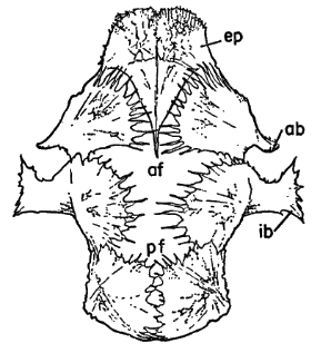
[Pg_401]
The angle η for any sector boundary can be found immediately by
measuring its position in the diagram (Figure 16). The form (Figure 18) for the "Computation of Zenith Distance and Azimuth of the
Moon" illustrates the steps in calculating the values of Z0 and ψ0.
From the American Air Almanac (Anonymous, 1945-1948), issued
annually by the U. S. Naval Observatory in three volumes, each
covering four months of the year, the Greenwich Hour Angle (GHA)
and the declination of the moon may be obtained for any ten-minute
interval of the date in question. The Local Hour Angle (LHA) of
the observation station is determined by subtracting the longitude
of the station from the GHA. Reference is then made to the
"Tables of Computed Altitude and Azimuth," published by the
U. S. Navy Department, Hydrographic Office (Anonymous, 1936-1941),
and better known as the "H.O. 214," to locate the altitude
and azimuth of the moon at the particular station for the middle
of the hour during which the observations were made. The tables
employ three variables—the latitude of the locality measured to
the nearest degree, the LHA as determined above, and the declination
of the moon measured to the nearest 30 minutes of arc.
Interpolations can be made, but this exactness is not required. When
the latitude of the observation station is in the northern hemisphere,
the H.O. 214 tables entitled "Declinations Contrary Name
to Latitude" are used with south declinations of the moon, and the
tables "Declinations Same Name as Latitude," with north declinations.
In the sample shown in Figure 15, the declination of the
moon at 11:30 P. M., midway through the 11 to 12 o'clock interval,
was S 20° 22´. Since the latitude of Progreso, Yucatán is N 21° 17´,
the "Contrary Name" tables apply to this hour.
Because the H.O. 214 expresses the vertical position of the moon
in terms of its altitude, instead of its zenith distance, a conversion
is required. The former is the number of arc degrees from the horizon
to the moon's center; therefore Z0 is readily obtained by subtracting
the altitude from 90°. Moreover, the azimuth given in the
H.O. 214 is measured on a 360° scale from the north point, whereas
the azimuth used here (ψ0) is measured 180° in either direction from
the south point, negative values to the east, positive values to the
west. I have designated the azimuth of the tables as Azn and obtained
the desired azimuth (ψ0) by subtracting 180° from Azn. The
sign of ψ0 may be either positive or negative, depending on whether
or not the moon has reached its zenith and hence the meridian of
the observer. When the GHA is greater than the local longitude
[Pg_402]
(that is, the longitude of the observation station), the azimuth is
positive. When the GHA is less than the local longitude, the
azimuth is negative.
Locating the position of a particular sector boundary now becomes
a mere matter of substituting the values in the equation (1)
and reducing. The computation of the north point for 11 to 12 P. M.
in the sample set of data will serve as an example. Since the north
point reckoned west from the south point is 180°, its η has a value
of 180°.
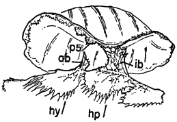
The example employed is the 11:00 to 12:00 P. M. diagram of Figure 15.
[Pg_403]
| tan θNpt. = | tan (180° - ψ0) |
| cos Z0 |
Substituting values of ψ0 found on the form (Figure 18):
| tan θNpt. = | tan [180° - (-35°)] | = | tan 215° | = | .700 | = 1.09 |
| cos 50° | cos 50° | .643 |
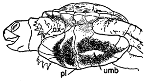
Four angles, one in each quadrant, have the same tangent value.
[Pg_404]
Since, in processing spring data, we are dealing mainly with north
sectors, it is convenient to choose the acute angle, in this instance
47°28´. In doubtful cases, the value of the numerator of the equation
(here 215°) applied as an angular measure from 6 o'clock will
tell in which quadrant the projected boundary must fall. The fact
that projection always draws the boundary closer to the 3-9 line
serves as a further check on the computation.
of the angle α
In the same manner, the projected position angles of all the pertinent
sector boundaries for a given hour may be calculated and plotted
in red pencil with a protractor on the circular diagrams of Figure 15. To avoid confusion in lines, the zones are not portrayed in the
black and white reproduction of the sample plot form. They are
shown, however, in the shaded enlargement (Figure 19) of the 11 to 12
P. M. diagram. The number of birds recorded for each sector may
be ascertained by counting the number of tally marks between each
pair of boundary lines and the information may be entered in the
columns provided in the plot form (Figure 15).
[Pg_405]
We are now prepared to turn to the form for "Computations of
Sector Densities" (Figure 20), which systematizes the solution of
the following equation:
(No. of Birds)(cos^2 Z_{0}))/(1 - sin^2 Z_{0} cos^2 [alpha])^0.5") | (2) |
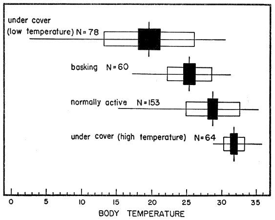
[Pg_406]
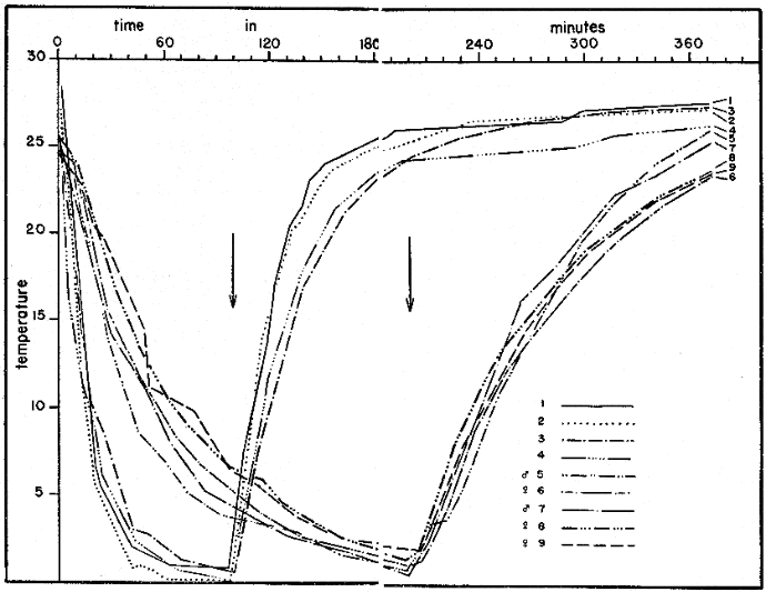
Some of the symbols and factors, appearing here for the first
time, require brief explanation. D stands for Sector Density. The
constant, 220, is the reciprocal of the quotient of the angular diameter
of the moon divided by 2. T is Time In, arrived at by subtracting
the total number of minutes of time out, as noted for each
hour on the original data sheets, from 60. "No. of Birds" is the
number for the sector and hour in question as just determined on
the plot form. The symbol represents the angle between the mid-line
of the sector and the azimuth line of the moon. The quantity
is found by the equation:
[Pg_407]
| α = 180° - η + ψ0 | (3) |
The symbol η here represents the position of the mid-line of the
sector expressed in terms of its 360° compass reading. This equation
is illustrated in Figure 21. The values of η for various zones are
given in the upper right-hand corner of the form (Figure 20). The
subsequent reductions of the equations, as they appear in the figure
for four zones, are self-explanatory. The end result, representing
the sector density, is entered in the rectangular box provided.
After all the sector densities have been computed, they are tabulated
on a form for the "Summary of Sector Densities" (Figure 22).
By totaling each vertical column, sums are obtained, expressing the
Station Density or Station Magnitude for each hour.
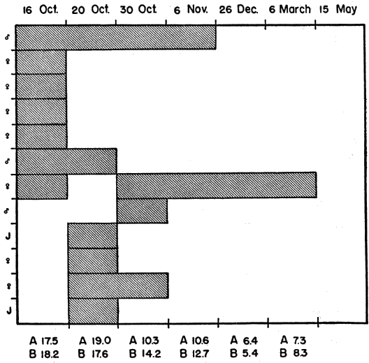
An informative way of depicting the densities in each zone is to
plot them as lines of thrust, as in Figure 23. Each sector is represented
by the directional slant of its mid-line drawn to a length expressing
the flight density per zone on some chosen scale, such as
100 birds per millimeter. Standard methods of vector analysis are
then applied to find the vector resultant. This is done by considering
the first two thrust lines as two sides of an imaginary parallelogram
and using a drawing compass to draw intersecting arcs locating
the position of the missing corner. In the same way, the third vector
[Pg_408]
is combined with the invisible resultant whose distal end is represented
by the intersection of the first two arcs. The process is repeated
successively with each vector until all have been taken into
consideration. The final intersection of arcs defines the length and
slant of the Vector Resultant, whose magnitude expresses the Net
Trend Density in terms of the original scale.
The final step in the processing of a set of observations is to plot
on graph paper the nightly station density curve as illustrated by
Figure 24.
Present day concepts of the whole broad problem of bird migration
are made up of a few facts and many guesses. The evolutionary
origin of migration, the modern necessities that preserve its biologic
utility, the physiological processes associated with it, the sensory
mechanisms that make it possible, the speed at which it is achieved,
and the routes followed, all have been the subject of some investigation
and much conjecture. All, to a greater or less extent, remain
matters of current controversy. All must be considered unknowns
in every logical equation into which they enter. Since all aspects of
the subject are intimately interrelated, since all have a bearing on
the probabilities relating to any one, and since new conjectures must
be judged largely in the light of old conjectures rather than against
a background of ample facts, the whole field is one in which many
alternative explanations of the established phenomena remain equally
tenable. Projected into this uncertain atmosphere, any statistical
approach such as determinations of flight density will require the
accumulation of great masses of data before it is capable of yielding
truly definitive answers to those questions that it is suited to solve.
Yet, even in their initial applications, density analyses can do much
to bring old hypotheses regarding nocturnal migration into sharper
definition and to suggest new ones.
The number of birds recorded through the telescope at a particular
station at a particular time is the product of many potential
variables. Some of these—like the changing size of the field of
observation and the elevation of flight—pertain solely to the capacity
of the observer to see what is taking place. It is the function
of the density and direction formulae to eliminate the influences of
these two variables insofar as is possible, so that the realities of the
situation take shape in a nearly statistically true form. There remain
to be considered those influences potentially responsible for
[Pg_409]
variations in the real volume of migration at different times and
places—things like the advance of season, geographic location,
disposition of terrain features, hourly activity rhythm, wind currents,
and other climatological causes. The situation represented
by any set of observations probably is the end result of the interaction
of several such factors. It is the task of the discussions that
follow to analyze flight densities in the light of the circumstances
surrounding them and by statistical insight to isolate the effects of
single factors. When this has been done, we shall be brought
closer to an understanding of these influences themselves as they
apply to the seasonal movements of birds. Out of data that is
essentially quantitative, conclusions of a qualitative nature will
begin to take form. It should be constantly borne in mind, however,
that such conclusions relate to the movement of birds en masse
and that caution must be used in applying these conclusions to
any one species.
Since the dispersal of migrants in the night sky has a fundamental
bearing on the sampling procedure itself, and therefore on the reliability
of figures on flight density, consideration can well be given
first to the horizontal distribution of birds on narrow fronts.
Bird migration, as we know it in daytime, is characterized by
spurts and uneven spatial patterns. Widely separated V's of geese
go honking by. Blackbirds pass in dense recurrent clouds, now on
one side of the observer, now on the other. Hawks ride along in
narrow file down the thermal currents of the ridges. Herons, in
companies of five to fifty, beat their way slowly along the line of the
surf. And an unending stream of swallows courses low along the
levees. Everywhere the impression is one of birds in bunches, with
vast spaces of empty sky between.
Such a situation is ill-suited to the sort of sampling procedure on
which flight density computations are based. If birds always
traveled in widely separated flocks, many such flocks might pass
near the cone of observation and still, by simple chance, fail to
enter the sliver of space where they could be seen. Chance would
be the dominating factor in the number of birds recorded, obscuring
the effects of other influences. Birds would seldom be seen, but,
when they did appear, a great many would be observed simultaneously
or in rapid succession.
[Pg_410]
When these telescopic studies were first undertaken at Baton
Rouge in 1945, some assurance already existed, however, that night
migrants might be so generally dispersed horizontally in the darkness
above that the number passing through the small segment of sky
where they could be counted would furnish a nearly proportionate
sample of the total number passing in the neighborhood of the
observation station. This assurance was provided by the very
interesting account of Stone (1906: 249-252), who enjoyed the
unique experience of viewing a nocturnal flight as a whole. On the
night of March 27, 1906, a great conflagration occurred in Philadelphia,
illuminating the sky for a great distance and causing the
birds overhead to stand out clearly as their bodies reflected the light.
Early in the night few birds were seen in the sky, but thereafter they
began to come in numbers, passing steadily from the southwest to
the northeast. At ten o'clock the flight was at its height. The
observer stated that two hundred birds were in sight at any given
moment as he faced the direction from which they came. This unparalleled
observation is of such great importance that I quote it in
part, as follows: "They [the birds] flew in a great scattered, wide-spread
host, never in clusters, each bird advancing in a somewhat
zigzag manner…. Far off in front of me I could see them
coming as mere specks…gradually growing larger as they
approached…. Over the illuminated area, and doubtless for
great distances beyond, they seemed about evenly distributed….
I am inclined to think that the migrants were not influenced
by the fire, so far as their flight was concerned, as those far
to the right were not coming toward the blaze but keeping steadily
on their way…. Up to eleven o'clock, when my observations
ceased, it [the flight] continued apparently without abatement, and
I am informed that it was still in progress at midnight."
Similarly, in rather rare instances in the course of the present
study, the combination of special cloud formations and certain atmospheric
conditions has made it possible to see birds across the
entire field of the telescope, whether they actually passed before the
moon or not. In such cases the area of the sky under observation is
greatly increased, and a large segment of the migratory movement
can be studied. In my own experience of this sort, I have been forcibly
impressed by the apparent uniformity and evenness of the procession
of migrants passing in review and the infrequence with which
birds appeared in close proximity.
As striking as these broader optical views of nocturnal migration
are, they have been too few to provide an incontestable basis for
[Pg_411]
generalizations. A better test of the prevailing horizontal distribution
of night migrants lies in the analysis of the telescopic data
themselves.
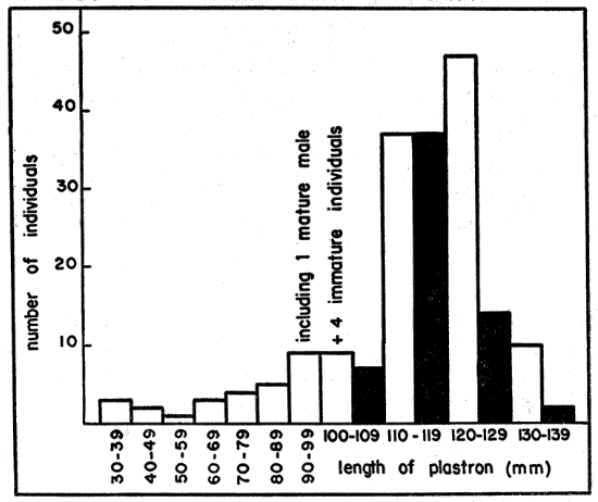
21-22, 1948. Essential features of this diagrammatic map are drawn to scale, the
triangular white lines representing the projections of the cone of observation
on the actual terrain at the mid-point of each hour of observation. If the
distal ends of the position lines were connected, the portion of the map encompassed
would represent the area over which all the birds seen between
8:30 P. M. and 3:30 A. M. must have flown.
The distribution in time of birds seen by a single observer may be
studied profitably in this connection. Since the cone of observation
is in constant motion, swinging across the front of birds migrating
from south to north, each interval of time actually represents a different
position in space. This is evident from the map of the progress
of the field of observation across the terrain at Tampico, Tamaulipas,
on April 21-22, 1948 (Figure 25). At this station on this
night, a total of 259 birds were counted between 7:45 P. M. and 3:45
[Pg_412]
A. M. The number seen in a single hour ranged from three to
seventy-three, as the density overhead mounted to a peak and then
declined. The number of birds seen per minute was not kept with
stop watch accuracy; consequently, analysis of the number of birds
that passed before the moon in short intervals of time is not justified.
It appears significant, however, that in the ninety minutes of heaviest
flight, birds were counted at a remarkably uniform rate per fifteen
minute interval, notwithstanding the fact that early in the period
the flight rate overhead had reached a peak and had begun to
decline. The number of birds seen in successive fifteen-minute periods
was twenty-six, twenty-five, nineteen, eighteen, fifteen, and
fifteen.
Also, despite the heavy volume of migration at this station on this
particular night, the flight was sufficiently dispersed horizontally so
that only twice in the course of eight hours of continuous observation
did more than one bird simultaneously appear before the moon.
These were "a flock of six birds in formation" seen at 12:09 A. M.
and "a flock of seven, medium-sized and distant," seen at 2:07 A. M.
In the latter instance, as generally is the case when more than one
bird is seen at a time, the moon had reached a rather low altitude,
and consequently the cone of observation was approaching its maximum
dimensions.
The comparative frequency with which two or more birds simultaneously
cross before the moon would appear to indicate whether
or not there is a tendency for migrants to fly in flocks. It is significant,
therefore, that in the spring of 1948, when no less than 7,432
observations were made of birds passing before the moon, in only
seventy-nine instances, or 1.1 percent of the cases, was more than
one seen at a time. In sixty percent of these instances, only two
birds were involved. In one instance, however, again when the
moon was low and the cone of observation near its maximum size,
a flock estimated at twenty-five was recorded.
The soundest approach of all to the study of horizontal distribution
at night, and one which may be employed any month, anywhere,
permitting the accumulation of statistically significant quantities
of data, is to set up two telescopes in close proximity. Provided
the flight overhead is evenly dispersed, each observer should
count approximately the same number of birds in a given interval
of time. Some data of this type are already available. On May 19-20,
at Urbana, Illinois, while stationed twenty feet apart making
parallax studies with two telescopes to determine the height above
[Pg_413]
the earth of the migratory birds, Carpenter and Stebbins (loci cit.)
saw seventy-eight birds in two and one-half hours. Eleven were
seen by both observers, thirty-three by Stebbins only, and thirty-four
by Carpenter only. On October 10, 1905, at the same place, in
two hours, fifty-seven birds were counted, eleven being visible
through both telescopes. Of the remainder, Stebbins saw seventeen
and Carpenter, twenty-nine. On September 12, 1945, at Baton
Rouge, Louisiana, in an interval of one hour and forty minutes, two
independent observers each counted six birds. Again, on October 17,
1945, two observers each saw eleven birds in twenty-two minutes.
On April 10, 1946, in one hour and five minutes, twenty-four birds
were seen through one scope and twenty-six through the other. Likewise
on May 12, 1946, in a single hour, seventy-three birds were
counted by each of two observers. The Baton Rouge observations
were made with telescopes six to twelve feet apart. These results
show a remarkable conformity, though the exceptional October observation
of Carpenter and Stebbins indicates the desirability of continuing
these studies, particularly in the fall.
On the whole, the available evidence points to the conclusion that
night migration differs materially from the kind of daytime migration
with which we are generally familiar. Birds are apparently
evenly spread throughout the sky, with little tendency to fly in
flocks. It must be remembered, however, that only in the case of
night migration have objective and truly quantitative studies been
made of horizontal distribution. There is a possibility that our impressions
of diurnal migration are unduly influenced by the fact
that the species accustomed to flying in flocks are the ones that attract
the most attention.
These conclusions relate to the uniformity of migration in terms
of short distances only, in the immediate vicinity of an observation
station. The extent to which they may be applied to broader fronts
is a question that may be more appropriately considered later, in
connection with continental aspects of the problem.
There are few aspects of nocturnal migration about which there is
less understanding than the matter of when the night flight begins,
at what rate it progresses, and for what duration it continues. One
would think, however, that this aspect of the problem, above most
others, would have been thoroughly explored by some means of
objective study. Yet, this is not the case. Indeed, I find not a
[Pg_414]
single paper in the American literature wherein the subject is discussed,
although some attention has been given the matter by
European ornithologists. Siivonen (1936) recorded in Finland the
frequency of call notes of night migrating species of Turdus and
from these data plotted a time curve showing a peak near midnight.
Bergman (1941) and Putkonen (1942), also in Finland, studied the
night flights of certain ducks (Clangula hyemalis and Oidemia fusca
and O. nigra) and a goose (Branta bernicla) and likewise demonstrated
a peak near midnight. However, these studies were made
at northern latitudes and in seasons characterized by evenings of
long twilight, with complete darkness limited to a period of short
duration around midnight. Van Oordt (1943: 34) states that in
many cases migration lasts all night; yet, according to him, most
European investigators are of the opinion that, in general, only a
part of the night is used, that is, the evening and early morning
hours. The consensus of American ornithologists seems to be that
migratory birds begin their flights in twilight or soon thereafter
and that they remain on the wing until dawn. Where this idea
has been challenged at all, the implication seems to have been that
the flights are sustained even longer, often being a continuation far
into the night of movements begun in the daytime. The telescopic
method fails to support either of these latter concepts.
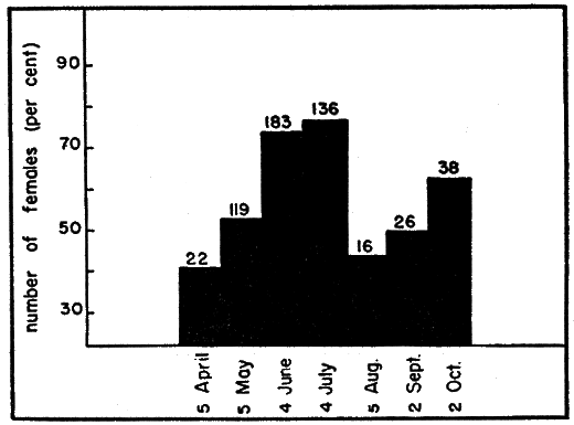
represents the arithmetic mean obtained by adding all the station densities
for each hour, regardless of date, and dividing the sum by the number of sets
of observations at that hour (CST).
When the nightly curves of density at the various stations are
plotted as a function of time, a salient fact emerges—that the flow
[Pg_415]
of birds is in no instance sustained throughout the night. The
majority of the curves rise smoothly from near zero at the time of
twilight to a single peak and then decline more or less symmetrically
to near the base line before dawn. The high point is reached in or
around the eleven to twelve o'clock interval more often than at any
other time.
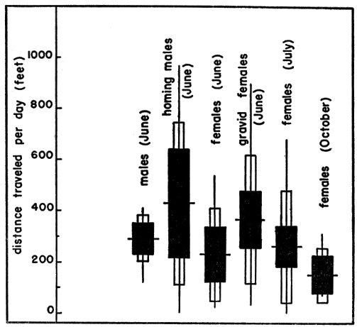
curve is based only on those sets of data where observations were continued
long enough to include the nightly peak. In each set of data the station
density for each hour has been expressed as a percentage of the peak for the
night at the station in question. All percentages for the same hour on all
dates have been averaged to obtain the percentile value of the combined
station density at each hour (CST).
Figure 26, representing the average hourly densities for all stations
on all nights of observation, demonstrates the over-all effect of
these tendencies. Here the highest density is reached in the hour
before midnight with indications of flights of great magnitude also
in the hour preceding and the hour following the peak interval.
The curve ascends somewhat more rapidly than it declines, which
fact may or may not be significant. Since there is a great disproportion
in the total volume of migration at different localities, the
thought might be entertained that a few high magnitude stations,
such as Tampico and Progreso, have imposed their own characteristics
on the final graph. Fortunately, this idea may be tested by
subjecting the data to a second treatment. If hourly densities are
expressed as a percentage of the nightly peak, each set of observations,
regardless of the number of birds involved, carries an equal
weight in determining the character of the over-all curve. Figure 27
shows that percentage analysis produces a curve almost identical
with the preceding one. To be sure, all of the individual curves do
not conform with the composite, either in shape or incidence of
[Pg_416]
peak. The extent of this departure in the latter respect is evident
from Figure 28, showing the number of individual nightly station
curves reaching a maximum peak in each hour interval. Even this
graph demonstrates that maximum densities near midnight represent
the typical condition.
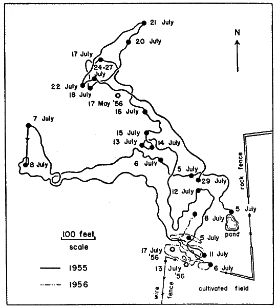
1948. "Number of stations" represents the total for all nights of the numbers
of station peaks falling within a given hour.
The remarkable smoothness and consistency of the curves shown
in Figures 26 and 27 seem to lead directly to the conclusion that
the volume of night migration varies as a function of time. Admittedly
other factors are potentially capable of influencing the
number of birds passing a given station in a given hour. Among
these are weather conditions, ecological patterns, and specific topographical
features that might conceivably serve as preferred avenues
of flight. However, if any of these considerations were alone
responsible for changes in the numbers of birds seen in successive
intervals, the distribution of the peak in time could be expected to
be haphazard. For example, there is no reason to suppose that the
cone of observation would come to lie over favored terrain at precisely
the hour between eleven and twelve o'clock at so many widely
separated stations. Neither could the topographical hypothesis explain
the consistently ascending and descending pattern of the ordinates
in Figure 28. This is not to say that other factors are without
effect; they no doubt explain the divergencies in the time pattern
exhibited by Figure 28. Nevertheless, the underlying circumstances
are such that when many sets of data are merged these other influences
are subordinated to the rise and fall of an evident time pattern.
[Pg_417]
Stated in concrete terms, the time frequencies shown in the graphs
suggest the following conclusions: first, nocturnal migrations are
not a continuation of daytime flights; second, nearly all night migrants
come to earth well before dawn; and, third, in each hour of
the night up until eleven or twelve o'clock there is typically a progressive
increase in the number of birds that have taken wing and
in each of the hours thereafter there is a gradual decrease. Taken at
its face value, the evidence seems to indicate that birds do not begin
their night migrations en masse and remain on the wing until dawn
and that in all probability most of them utilize less than half of the
night.
Interestingly enough, the fact that the plot points in Figure 26
lie nearly in line tempts one to a further conclusion. The curve behaves
as an arithmetic progression, indicating that approximately
the same number of birds are leaving the ground in each hour interval
up to a point and that afterwards approximately the same number
are descending within each hour. However, some of the components
making up this curve, as later shown, are so aberrant in
this regard that serious doubt is cast on the validity of this generalization.
Because the results of these time studies are unexpected and startling,
I have sought to explore other alternative explanations and
none appears to be tenable. For example, the notion that the varying
flight speeds of birds might operate in some way to produce a
cumulative effect as the night progresses must be rejected on close
analysis. If birds of varying flight speeds are continuously and
evenly distributed in space, a continuous and even flow would result
all along their line of flight. If they are haphazardly distributed in
space, a correspondingly haphazard density pattern would be expected.
Another explanation might be sought in the purely mathematical
effects of the method itself. The computational procedure assumes
that the effective area of the sample is extremely large when the
moon is low, a condition that usually obtains in the early hours of
the evening in the days surrounding the full moon. Actually no
tests have yet been conducted to ascertain how far away a silhouette
of a small bird can be seen as it passes before the moon. Consequently,
it is possible that some birds are missed under these conditions
and that the effective field of visibility is considerably smaller
than the computed field of visibility. The tendency, therefore, may
be to minimize the densities in such situations more than is justified.
[Pg_418]
However, in many, if not most, cases, the plotting of the actual
number of birds seen, devoid of any mathematical procedures, results
in an ascending and descending curve.
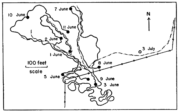
April 22-23; (B) random fluctuation, Stillwater, April 23-24; (C) bimodal,
Knoxville, April 22-23; (D) sustained peak, Ottumwa, April 21-22; (E) early
peak, Oak Grove, May 21-22; (F) late peak, Memphis, April 23-24.
A third hypothesis proposes that all birds take wing at nearly the
same time, gradually increase altitude until they reach the mid-point
of their night's journey, and then begin a similarly slow descent.
Since the field of observation of the telescope is conical, it is assumed
that the higher the birds arise into the sky the more they increase
their chances of being seen. According to this view, the changes
[Pg_419]
in the density curve represent changes in the opportunity to see
birds rather than an increase or decrease in the actual number of
migrants in the air. Although measurements of flight altitude at
various hours of the night have not been made in sufficient number
to subject this idea to direct test, it is hardly worthy of serious
consideration. The fallacy in the hypothesis is that the cone of
observation itself would be rising with the rising birds so that
actually the greatest proportion of birds flying would still be seen
when the field of observation is in the supine position of early
evening.
It cannot be too strongly emphasized that the over-all time
curves just discussed have been derived from a series of individual
curves, some of which differ radically from the composite pattern.
In Figure 29, six dissimilar types are shown. This variation is not
surprising in view of the fact that many other causative factors
aside from time operate on the flow of birds from hour to hour.
Figure 29A illustrates how closely some individual patterns conform
with the average. Figure 29B is an example of a random type
of fluctuation with no pronounced time character. It is an effect
rarely observed, occurring only in the cases where the number of
birds observed is so small that pure chance has a pronounced effect
on the computed densities; its vacillations are explicable on that
account alone. Errors of sampling may similarly account for some,
though not all, of the curves of the bimodal type shown in Figure 29C.
Some variation in the curves might be ascribed to the variations
in kinds of species comprising the individual flights at different
times at different places, provided that it could be demonstrated
that different species of birds show dissimilar temporal patterns.
The other atypical patterns are not so easily dismissed and will be
the subject of inquiry in the discussions that follow. It is significant
that in spite of the variety of the curves depicted, which represent
every condition encountered, in not a single instance is the density
sustained at a high level throughout the night. Moreover, these
dissident patterns merge into a remarkably harmonious, almost
normal, average curve.
When, at some future date, suitable data are available, it would
be highly desirable to study the average monthly time patterns to
ascertain to what extent they may deviate from the over-all average.
At present this is not justifiable because there are not yet enough
sets of data in any two months representing the same selection of
stations.
It is especially interesting to note that the data pertaining to this
problem derived from other methods of inquiry fit the conclusions
adduced by the telescopic method. Overing (1938), who for several
years kept records of birds striking the Washington Monument,
stated that the record number of 576 individuals killed on the night
of September 12, 1937, all came down between 10:30 P. M. and midnight.
His report of the mortality on other nights fails to mention
the time factor, but I am recently informed by Frederick C. Lincoln
(in litt.) that it is typical for birds to strike the monument in
greatest numbers between ten and twelve o'clock at night. At the
latter time the lights illuminating the shaft are extinguished, thus
resulting in few or no casualties after midnight. The recent report
by Spofford (1949) of over 300 birds killed or incapacitated at the
Nashville airport on the night of September 9-10, 1948, after flying
into the light beam from a ceilometer, is of interest in this connection
even though the cause of the fatality is shrouded in mystery.
It may be noted, however, that "most of the birds fell in the first
hour," which, according to the account, was between 12:30 A. M. and
1:30 A. M. Furthermore, birds killed at the Empire State Building in
New York on the night of September 10-11, 1948, began to strike
the tower "shortly after midnight" (Pough, 1948). Also it will be
recalled that the observations of Stone (loc. cit.), already referred
to in this paper (page 410), show a situation where the flight in the
early part of the night was negligible but mounted to a peak between
ten and eleven o'clock, with continuing activity at least until
midnight.
All of these observations are of significance in connection with
the conclusions herein advanced, but by far the most striking correlation
between these present results and other evidences is found
in the highly important work of various European investigators
studying the activity of caged migratory birds. This work was
recently reviewed and extended by Palmgren (1944) in the most
comprehensive treatise on the subject yet published. Palmgren recorded,
by an electrically operated apparatus, the seasonal, daily,
and hourly activity patterns in caged examples of two typical
European migrants, Turdus ericetorum philomelos Brehm and Erithacus
rubecula (Linnaeus). Four rather distinct seasonal phases
in activity of the birds were discerned: winter non-migratory,
spring migratory, summer non-migratory, and autumn migratory.
The first of these is distinguished by morning and evening maxima
[Pg_421]
of activity, the latter being better developed but the former being
more prolonged. Toward the beginning of migration, these two periods
of activity decline somewhat. The second, or spring migratory
phase, which is of special interest in connection with the present
problem, is characterized by what Palmgren describes as nightly
migratory restlessness (Zugunruhe). The morning maximum, when
present, is weaker and the evening maximum often disappears altogether.
Although variations are described, the migratory restlessness
begins ordinarily after a period of sleep ("sleeping pause") in
the evening and reaches a maximum and declines before midnight.
This pattern agrees closely with the rhythm of activity indicated
by the time curves emerging from the present research. Combining
the two studies, we may postulate that most migrants go to sleep for
a period following twilight, thereby accounting for the low densities
in the early part of the night. On awakening later, they begin to
exhibit migratory restlessness. The first hour finds a certain number
of birds sufficiently stimulated so that they rise forthwith into
the air. In the next hour still others respond to this urge and they
too mount into the air. This continues until the "restlessness" begins
to abate, after which fewer and fewer birds take wing. By this
time, the birds that began to fly early are commencing to descend,
and since their place is not being filled by others leaving the ground,
the density curve starts its decline. Farner (1947) has called attention
to the basic importance of the work by Palmgren and the many
experimental problems it suggests. Of particular interest would be
studies comparing the activity of caged American migrant species
and the nightly variations in the flight rates.
As already stated, the present study was initiated at Baton Rouge,
Louisiana, in 1945, and from the outset a very peculiar density time
pattern was manifest. I soon found that birds virtually disappeared
from the sky after midnight. Within an hour after the termination
of twilight, the density would start to ascend toward a peak which
was usually reached before ten o'clock, and then would begin, surprisingly
enough, a rapid decline, reaching a point where the migratory
flow was negligible. In Figure 30 the density curves are shown for
five nights that demonstrate this characteristically early decline in
the volume of migration at this station. Since, in the early stages
of the work, coördinates of apparent pathways of all the birds seen
were not recorded, I am unable now to ascertain the direction of
flight and thereby arrive at a density figure based on the dimension
of the cone and the length of the front presented to birds flying in
certain directions. It is feasible, nevertheless, to compute what I
have termed a "plus or minus" flight density figure stating the rate
of passage of birds in terms of the maximum and minimum corrections
which all possible directions of flight would impose. In other
words, density is here computed, first, as if all the birds were flying
perpendicular to the long axis of the ellipse, and, secondly, as if all
the birds were flying across the short axis of the ellipse. Since the
actual directions of flight were somewhere between these two extremes,
the "plus or minus" density figure is highly useful.
[Pg_422]
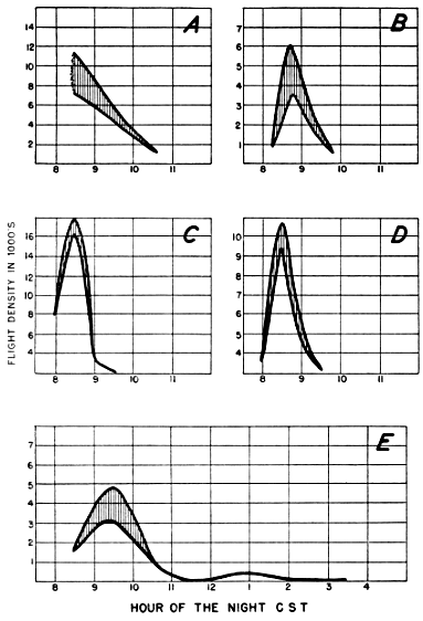
25, 1945; (B) April 15, 1946; (C) May 10, 1946; (D) May 15, 1946; (E) April
22-23, 1948. These curves are plotted on a "plus or minus" basis as described in
the text, with the bottom of the curve representing the minimum density and
the top of the curve the maximum.
[Pg_423]
The well-marked decline before midnight in the migration rates
at Baton Rouge may be regarded as one of the outstanding results
emerging from this study. Many years of ornithological investigation
in this general region failed to suggest even remotely that a
situation of this sort obtained. Now, in the light of this new fact,
it is possible for the first time to rationalize certain previously incongruous
data. Ornithologists in this area long have noted that
local storms and cold-front phenomena at night in spring sometimes
precipitate great numbers of birds, whereupon the woods are filled
the following day with migrants. On other occasions, sudden storms
at night have produced no visible results in terms of bird densities
the following day. For every situation such as described by Gates
(1933) in which hordes of birds were forced down at night by inclement
weather, there are just as many instances, even at the height
of spring migration, when similar weather conditions yielded no
birds on the ground. However, the explanation of these facts is
simple; for we discover that storms that produced birds occurred
before midnight and those that failed to produce birds occurred after
that time (the storm described by Gates occurred between 8:30 and
9:00 P. M.).
The early hour decline in density at Baton Rouge at first did not
seem surprising in view of the small amount of land area between
this station and the Gulf of Mexico. Since the majority of the
birds destined to pass Baton Rouge on a certain night come in
general from the area to the south of that place, and since the
distances to various points on the coast are slight, we inferred
that a three-hour flight from even the more remote points would
probably take the bulk of the birds northward past Baton Rouge.
In short, the coastal plain would be emptied well before midnight
of its migrant bird life, or at least that part of the population destined
to migrate on any particular night in question. Although data
[Pg_424]
in quantity are not available from stations on the coastal plain other
than Baton Rouge, it may be pointed out that such observations as
we do have, from Lafayette and New Orleans, Louisiana, and from
Thomasville, Georgia, are in agreement with this hypothesis.
A hundred and seventy miles northward in the Mississippi Valley,
at Oak Grove, Louisiana, a somewhat more normal density pattern
is manifested. There, in four nights of careful observation, a pronounced
early peak resulted on the night of May 21-22 (Figure 29E),
but on the other three nights significant densities held up until
near twelve o'clock, thereby demonstrating the probable effect of
the increased amount of land to the south of the station.
Subsequent studies, revealing the evident existence of an underlying
density time pattern, cast serious doubt on the explanations
just advanced of the early decline in the volume of migration at
Baton Rouge. It has as yet been impossible to reconcile the early
drop-off at this station with the idea that birds are still mounting
into the air at eleven o'clock, as is implied by the ideal time curves.
To this point we have considered the horizontal distribution of
birds in the sky only on a very narrow scale and mainly in terms
of the chance element in observations. Various considerations have
supported the premise that the spread of nocturnal migration is
rather even, at least within restricted spacial limits and short intervals
of time. This means that in general the flow of birds from
hour to hour at a single station exhibits a smooth continuity. It
does not mean that it is a uniform flow in the sense that approximately
the same numbers of birds are passing at all hours, or at all
localities, or even on all one-mile fronts in the same locality. On the
contrary, there is evidence of a pronounced but orderly change
through the night in the intensity of the flight, corresponding to a
basic and definitely timed cycle of activity. Other influences may
interfere with the direct expression of this temporal rhythm as it
is exhibited by observations at a particular geographical location.
Among these, as we have just seen, is the disposition of the areas
that offer suitable resting places for transient birds and hence contribute
directly and immediately to the flight overhead. A second
possible geographical effect is linked with the question of the tendency
of night migrants to follow topographical features.
That many diurnal migrants tend to fly along shorelines, rivers,
[Pg_425]
and mountain ridges is well known, but this fact provides no assurance
that night migrants do the same thing. Many of the obvious
advantages of specialized routes in daylight, such as feeding opportunities,
the lift provided by thermal updrafts, and the possible
aid of certain landmarks in navigation, assume less importance after
night falls. Therefore, it would not be safe to conclude that all
nocturnal migrants operate as do some diurnal migrants. For instance,
the passage of great numbers of certain species of birds along
the Texas coast in daylight hours cannot be regarded as certain
proof that the larger part of the nocturnal flight uses the same route.
Neither can we assume that birds follow the Mississippi River at
night simply because we frequently find migrants concentrated along
its course in the day. Fortunately we shall not need to speculate
indefinitely on this problem; for the telescopic method offers a means
of study based on what night migrants are doing at night. Two
lines of attack may be pursued. First we may compare flight
densities obtained when the field of the telescope lies over some outstanding
topographical feature, such as a river, with the recorded
volume of flight when the cone of observation is directed away from
that feature. Secondly, we may inquire how the major flight directions
at a certain station are oriented with respect to the terrain.
If the flight is concentrated along a river, for instance, the flight
density curve should climb upward as the cone of observation swings
over the river, regardless of the hour at which it does so. The effect
should be most pronounced if the observer were situated on the river
bank, so that the cone would eventually come to a position directly
along the watercourse. Though in that event birds coming up the
river route would be flying across the short axis of an elliptical section
of the cone, the fact that the whole field of observation would be
in their path should insure their being seen in maximum proportions.
If, on the other hand, the telescope were set up some distance away
from the river so that the cone merely moved across its course, only
a section of the observation field would be interposed on the main
flight lane.
The interaction of these possibilities with the activity rhythm
should have a variety of effects on the flight density curves. If the
cone comes to lie over the favored topographical feature in the hour
of greatest migrational activity, the results would be a simple sharp
peak of doubtful meaning. However, since the moon rises at a different
time each evening, the cone likewise would reach the immediate
[Pg_426]
vicinity of the terrain feature at a different time each night.
As a result, the terrain peak would move away from its position of
coincidence with the time peak on successive dates, producing first,
perhaps, a sustention of peak and later a definitely bimodal curve.
Since other hypotheses explain double peaks equally well, their
mere existence does not necessarily imply that migrants actually
do travel along narrow topographical lanes. Real proof requires
that we demonstrate a moving peak, based on properly corrected
density computations, corresponding always with the position of the
cone over the most favored terrain, and that the flight vectors be
consistent with the picture thus engendered.
To date, none of the evidence in favor of the topographical hypothesis
completely fills these requirements. Winkenwerder (loc. cit.),
in analyzing the results of telescopic counts of birds at Madison and
Beloit, Wisconsin, Detroit and Ann Arbor, Michigan, and at Lake
Forest, Illinois, between 1898 and 1900, plotted the number of birds
seen at fifteen-minute intervals as a function of the time of the night.
He believed that the high points in the resulting frequency histograms
represented intervals when the field of the telescope was
moving over certain topographically determined flight lanes, though
he did not specify in all cases just what he assumed the critical
physiographic features to be. Especially convincing to him were
results obtained at Beloit, where the telescope was situated on the
east bank of the Rock River, on the south side of the city. Immediately
below Beloit the river turns southwestward and continues
in this direction about five miles before turning again to flow in a
southeastward course for approximately another five miles. In this
setting, on two consecutive nights of observation in May, the number
of birds observed increased tremendously in the 2 to 3 A. M. interval,
when, according to Winkenwerder's interpretation of the data (he
did not make the original observations at Beloit himself), the telescope
was pointing directly down the course of the river. This conclusion
is weakened, however, by notable inconsistencies. Since
the moon rises later each evening, it could not have reached the
same position over the Rock River at the same time on both May
12-13 and May 13-14, and therefore, if the peaks in the graph were
really due to a greater volume of migration along the watercourse,
they should not have so nearly coincided. As a matter of fact the
incidence of the peak on May 12-13 should have preceded that of
[Pg_427]
the peak on May 13-14; whereas his figure shows the reverse to
have been true. Singularly enough, Winkenwerder recognized this
difficulty in his treatment of the data from Madison, Wisconsin.
Unable to correlate the peak period with the Madison terrain by the
approach used for Beloit, he plotted the observations in terms of
hours after moonrise instead of standard time. This procedure was
entirely correct; the moon does reach approximately the same position
at each hour after its rise on successive nights. The surprising
thing is that Winkenwerder did not seem to realize the incompatibility
of his two approaches or to realize that he was simply choosing
the method to suit the desired results.
Furthermore, as shown in Part I of this paper, the number of birds
seen through the telescope often has only an indirect connection with
the actual number of birds passing over. My computations reveal
that the highest counts of birds at Beloit on May 12-13 were recorded
when the moon was at an altitude of only 8° to 15° and, that
when appropriate allowance is made for the immense size of the field
of observation at this time, the partially corrected flight density for
the period is not materially greater than at some other intervals
in the night when the telescope was not directed over the course of
the Rock River. These allowances do not take the direction factor
into consideration. Had the birds been flying at right angles to the
short axis of an elliptical section of the cone throughout the night, the
flight density in the period Winkenwerder considered the peak would
have been about twice as high as in any previous interval. On the
other hand, if they had been flying across the long axis at all times,
the supposed peak would be decidedly inferior to the flight density
at 10 to 11:00 P. M., before the cone came near the river.
Admittedly, these considerations contain a tremendous element of
uncertainty. They are of value only because they expose the equal
uncertainty in Winkenwerder's basic evidence. Since the coördinates
of the birds' apparent pathways at Beloit were given, I at
first entertained the hope of computing the flight densities rigorously,
by the method herein employed. Unfortunately, Winkenwerder
was apparently dealing with telescopes that gave inverted images,
and he used a system for recording coördinates so ambiguously described
that I am not certain I have deciphered its true meaning.
When, however, his birds are plotted according to the instructions
as he stated them, the prevailing direction of flight indicated by the
projection formula falls close to west-northwest, not along the course
of the Rock River, but at direct right angles to it.
[Pg_428]
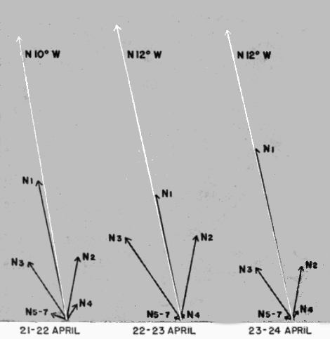
densities expressed as a percentage of the station density for that night; the
vector resultants are plotted from them by standard procedure. Thus, the
nightly diagrams are not on the same scale with respect to the actual number
of birds involved.
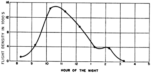
I am in a position to establish more exact correlations between
flight density and terrain features in the case of current sets of
observations. Some of these data seem at first glance to fit the idea
of narrow topographically-oriented flight lanes rather nicely. At
Tampico, where six excellent sets of observations were made in
March and April, 1948, the telescope was set up on the beach within
a few yards of the Gulf of Mexico. As can be seen from Figure 25
(ante), the slant of the coastline at this point is definitely west of
north, as is also the general trend of the entire coast from southern
Veracruz to southern Tamaulipas (see Figure 34, beyond). The
[Pg_429]
over-all vector resultant of all bird flights at this station was
N 11° W, and, as will be seen from Figure 31, none of the nightly
vector resultants in April deviates more than one degree from this
average. Thus the prevailing direction of flight, as computed, agrees
with the trend of the coast at the precise point of the observations,
at least to the extent that both are west of north. To be sure, the
individual sector vectors indicate that not all birds were following
this course; indeed, some appear to have been flying east of north,
heading for a landfall in the region of Brownsville, Texas, and a
very few to have been traveling northeastward toward the central
Gulf coast. But it must be remembered that a certain amount of
computational deviation and of localized zigzagging in flight must be
anticipated. Perhaps none of these eastward vectors represents an
actual extended flight path. The nightly vector resultants, on the
other hand, are so consistent that they have the appearance of remarkable
accuracy and tempt one to draw close correlations with the
terrain. When this is done, it is found that, while the prevailing
flight direction is 11° west of north, the exact slant of the coastline at
the location of the station is about 30° west of north, a difference of
around 19°. It appears, therefore, that the birds were not following
the shoreline precisely but cutting a chord about ten miles long across
an indentation of the coast. If it be argued that the method of
calculation is not accurate enough to make a 19° difference significant,
and that most of the birds might have been traveling along
the beach after all, it can be pointed out with equal justification
that, if this be so, the 11° divergence from north does not mean
anything either and that perhaps the majority of the birds were
[Pg_430]
going due north. We are obliged to conclude either that the main
avenue of flight paralleled the disposition of the major topographical
features only in a general way or that the angle between the line of
the coast and true north is not great enough to warrant any inference
at all.
Consideration of the Tampico density curves leads to similarly
ambiguous results. On the night of April 21-22, as is evident from
a comparison of Figures 25 and 32, the highest flight density occurred
when the projection of the cone on the terrain was wholly
included within the beach. This is very nearly the case on the night
of April 23-24 also, the positions of the cone during the peak period
of density being only about 16° apart. (On the intervening date,
clouds prevented continuous observation during the critical part of
the night.) These correlations would seem to be good evidence that
most of these night migrants were following the coastline of the
Gulf of Mexico. However, the problem is much more complicated.
The estimated point of maximum flight density fell at 10:45 P. M.
on April 21-22 and 11:00 P. M. on April 23-24, both less than an hour
from the peak in the ideal time curve (Figure 26, ante). We cannot
be sure, therefore, that the increase in density coinciding with the
position of the moon over the beach is not an increase which would
have occurred anyway. Observations conducted several nights
before or after the second quarter, when the moon is not on or near
its zenith at the time of the predictable peak in the density curve,
would be of considerable value in the study of this particular
problem.
The situation at Tampico has been dealt with at length because,
among all the locations for which data are available, it is the one
that most strongly supports the topographical hypothesis. In none
of the other cases have I been able to find a definite relation between
the direction of migration and the features of the terrain. Studies
of data from some of these stations disclose directional patterns that
vary from night to night only slightly more than does the flight at
Tampico. In three nights of observation at Lawrence, Kansas,
marked by very high densities, the directional trend was north by
north-northeast with a variation of less than 8°, yet Lawrence is so
situated that there seems to be no feature of the landscape locally
or in the whole of eastern Kansas or of western Missouri that coincides
with this heading. At Mansfield, Louisiana, in twelve nights
of observation, the strong east by northeast trend varied less than
15°, but again there appears to be no correlation over a wide area
[Pg_431]
between this direction and any landmarks. And, at Progreso, Yucatán,
where the vector resultants were 21° and 27° on successive
nights, most of the birds seen had left the land and were beginning
their flight northward over the trackless waters of the Gulf of Mexico.
Furthermore, as I have elsewhere pointed out (1946: 205), the
whole northern part of the Yucatán Peninsula itself is a flat terrain,
unmarked by rivers, mountains, or any other strong physiographic
features that conceivably might be followed by birds.
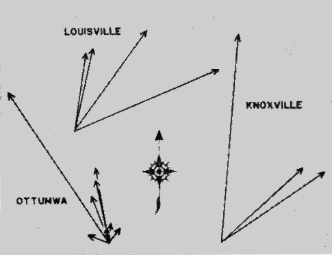
Each arrow is the vector resultant for a particular night, its length expressing the
nightly density as a percentage of the total station density for the nights represented.
Thus, the various station diagrams are not to the same scale.
In Figure 33 I have shown the directional patterns at certain stations
where, unlike the cases noted above, there is considerable
change on successive nights. Each vector shown is the vector resultant
for one particular night. The lengths of the vectors have been
determined by their respective percentages of the total computed
density, or total station magnitude, for all the nights in question.
In other words, the lengths of the individual vectors denote the percentile
rôle that each night played in the total density. From the
directional spread at these stations it becomes apparent that if most
of the birds were traveling along a certain topographic feature on one
[Pg_432]
night, they could not have been traveling along the same feature on
other nights.
The possibility should be borne in mind, however, that there may
be more than one potential topographic feature for birds to follow
at some stations. Moreover, it is conceivable that certain species
might follow one feature that would lead them in the direction of
their ultimate goal, whereas other species, wishing to go in an entirely
different direction, might follow another feature that would
lead them toward their respective destination. It would seem unlikely,
however, that the species composition of the nocturnal flights
would change materially from night to night, although there is a
strong likelihood that it might do so from week to week and certainly
from month to month.
By amassing such data as records of flight direction along the
same coast from points where the local slant of the shoreline is
materially different, and comparisons of the volume of migration at
night along specialized routes favored during the day with the flight
densities at progressive distances from the critical terrain feature
involved, we shall eventually be able to decide definitely the rôle
topography plays in bird migration. We cannot say on the basis of
the present ambiguous evidence that it is not a factor in determining
which way birds fly, but, if I had to hazard a guess one way or the
other, I would be inclined to discount the likelihood of its proving
a major factor.
Pattern
A study of the total nightly or seasonal densities at the various
stations brings forth some extremely interesting factors, many of
which, however, cannot be fully interpreted at this time. A complete
picture of the magnitude of migration at a given station cannot
be obtained from the number of birds that pass the station on
only a few nights in one spring. Many years of study may be required
before hard and fast principles are justifiable. Nevertheless,
certain salient features stand out in the continental density pattern
in the spring of 1948. (The general results are summarized in
Tables 2-5; the location of the stations is shown in Figure 34.)
These features will be discussed now on a geographical basis.
[Pg_433]
| Observation Station | Nights of observation | Hours of observation | Season density | ||||||
| March | April | May | Total | March | April | May | Total | ||
| Canada | |||||||||
| Pt. Pelee | 1 | 1 | 6 | 6 | 2,500 | ||||
| Mexico | |||||||||
| S. L. P.: Ebano | 1 | 1 | 3 | 3 | 1,300 | ||||
| Tamps.: Tampico | 3 | 3 | 6 | 20 | 20 | 40 | 140,300 | ||
| Yuc.: Progreso | 3 | 3 | 18 | 18 | 60,500 | ||||
| United States | |||||||||
| Fla.: Pensacola | 2 | 2 | 4 | 8 | 7 | 15 | 1,500 | ||
| Winter Park | 5 | 6 | 11 | 39 | 38 | 77 | 21,700 | ||
| Ga.: Athens | 2 | 2 | 10 | 10 | 4,000 | ||||
| Thomasville | 1 | 1 | 2 | 8 | 8 | 16 | 4,700 | ||
| Iowa: Ottumwa | 5 | 5 | 10 | 16 | 28 | 44 | 134,400 | ||
| Kans.: Lawrence | 2 | 1 | 3 | 16 | 4 | 20 | 68,700 | ||
| Ky.: Louisville | 3 | 2 | 5 | 20 | 14 | 34 | 49,300 | ||
| Murray | 2 | 2 | 13 | 13 | 26,200 | ||||
| La.: Baton Rouge | 3 | 3 | 15 | 15 | 11,000 | ||||
| Lafayette | 1 | 1 | 5 | 5 | 2,800 | ||||
| Mansfield | 1 | 5 | 4 | 10 | 2 | 16 | 22 | 40 | 22,400 |
| New Orleans | 1 | 1 | 2 | 5 | 2 | 7 | 1,900 | ||
| Oak Grove | 2 | 2 | 4 | 16 | 15 | 31 | 33,900 | ||
| Mich.: Albion | 1 | 1 | 3 | 3 | 1,100 | ||||
| Minn.: Hopkins | 1 | 1 | 4 | 4 | 2,000 | ||||
| Miss.: Rosedale | 1 | 1 | 2 | 6 | 8 | 14 | 12,600 | ||
| Mo.: Columbia | 2 | 1 | 3 | 8 | 6 | 14 | 13,100 | ||
| Liberty | 1 | 1 | 2 | 7 | 7 | 14 | 4,800 | ||
| Okla.: Stillwater | 1 | 2 | 1 | 4 | 5 | 11 | 3 | 19 | 8,400 |
| S. Car.: Charleston | 1 | 1 | 1 | 3 | 5 | 8 | 9 | 22 | 3,000 |
| Tenn.: Knoxville | 2 | 2 | 4 | 18 | 14 | 32 | 35,400 | ||
| Memphis | 2 | 3 | 2 | 7 | 13 | 20 | 12 | 45 | 29,700 |
| Tex.: College Station | 3 | 1 | 4 | 19 | 8 | 27 | 32,200 | ||
| Rockport | 1 | 1 | 4 | 4 | 6,200 | ||||
[Pg_434]
| Observation Station | March | April | May | Season |
| Canada | ||||
| Pt. Pelee | 400 | 400 | ||
| Mexico | ||||
| S. L. P.: Ebano | 400 | 400 | ||
| Tamps.: Tampico | 700 | 6,300 | 3,500 | |
| Yuc.: Progreso | 2,800 | 2,800 | ||
| United States | ||||
| Fla.: Pensacola | 0+ | 200 | 100 | |
| Winter Park | 300 | 200 | 300 | |
| Ga.: Athens | 400 | 400 | ||
| Thomasville | 500 | 100 | 300 | |
| Iowa: Ottumwa | 1,700 | 3,800 | 3,100 | |
| Kans.: Lawrence | 4,000 | 1,400 | 3,400 | |
| Ky.: Louisville | 2,000 | 700 | 1,500 | |
| Murray | 2,000 | 2,000 | ||
| La.: Baton Rouge | 700 | 700 | ||
| Lafayette | 600 | 600 | ||
| Mansfield | 0 | 700 | 800 | 600 |
| New Orleans | 60 | 800 | 300 | |
| Oak Grove | 1,400 | 800 | 1,100 | |
| Mich.: Albion | 400 | 400 | ||
| Minn.: Hopkins | 500 | 500 | ||
| Miss.: Rosedale | 1,100 | 700 | 900 | |
| Mo.: Columbia | 400 | 1,700 | 900 | |
| Liberty | 500 | 200 | 300 | |
| Okla.: Stillwater | 500 | 200 | 1,000 | 400 |
| S. Car.: Charleston | 200 | 200 | 0+ | 100 |
| Tenn.: Knoxville | 1,300 | 800 | 1,100 | |
| Memphis | 300 | 800 | 900 | 700 |
| Tex.: College Station | 1,100 | 1,500 | 1,200 | |
| Rockport | 1,600 | 1,600 |
[Pg_435]
| Observation Station | March | April | May |
| Canada | |||
| Pt. Pelee | 1,400 | ||
| Mexico | |||
| S. L. P.: Ebano | 600 | ||
| Tamps.: Tampico | 3,100 | 21,200 | |
| Yuc.: Progreso | 11,900 | ||
| United States | |||
| Fla.: Pensacola | 100 | 700 | |
| Winter Park | 2,300 | 1,000 | |
| Ga.: Athens | 900 | ||
| Thomasville | 1,500 | 200 | |
| Iowa: Ottumwa | 3,800 | 12,500 | |
| Kans.: Lawrence | 14,500 | 2,200 | |
| Ky.: Louisville | 5,000 | 1,400 | |
| Murray | 3,700 | ||
| La.: Baton Rouge | 3,400 | ||
| Lafayette | 1,800 | ||
| Mansfield | 2,100 | 1,600 | |
| New Orleans | 200 | 1,100 | |
| Oak Grove | 2,700 | 2,500 | |
| Mich.: Albion | 700 | ||
| Minn.: Hopkins | 1,100 | ||
| Miss.: Rosedale | 2,200 | 1,400 | |
| Mo.: Columbia | 800 | 3,400 | |
| Liberty | 800 | 800 | |
| Okla.: Stillwater | 900 | 700 | 1,400 |
| S. Car.: Charleston | 400 | 600 | 200 |
| Tenn.: Knoxville | 5,800 | 1,900 | |
| Memphis | 1,200 | 3,400 | 2,100 |
| Tex.: College Station | 3,400 | 3,100 | |
| Rockport | 2,400 |
[Pg_436]
| Observation Station | March | April | May |
| Mexico | |||
| Tamps.: Tampico | 5,500 | 63,600 | |
| Yuc.: Progreso | 31,600 | ||
| United States | |||
| Fla.: Winter Park | 6,200 | ||
| Ga.: Athens | 2,600 | ||
| Thomasville | 3,900 | ||
| Iowa: Ottumwa | 15,300 | 54,600 | |
| Kans.: Lawrence | 51,600 | 5,400 | |
| Ky.: Louisville | 17,000 | 8,400 | |
| Murray | 16,400 | ||
| La.: Baton Rouge | 6,200 | ||
| Mansfield | 4,900 | 5,200 | |
| Oak Grove | 13,600 | 5,800 | |
| Miss.: Rosedale | 6,800 | 5,800 | |
| Mo.: Columbia | 1,400 | 10,300 | |
| Okla.: Stillwater | 2,700 | 1,900 | 3,000 |
| Tenn.: Knoxville | 15,200 | 9,000 | |
| Memphis | 3,600 | 7,900 | 7,000 |
| Tex.: College Station | 6,200 | 13,200 |
[Pg_437]
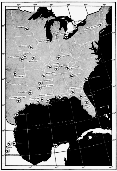
[Pg_438]
In view of the controversy in recent years pertaining to migration
routes in the region of the Gulf of Mexico (Williams, 1945 and 1947;
Lowery, 1945 and 1946), the bearing of the new data on the problem
is of especial interest. While recent investigations have lent
further support to many of the ideas expressed in my previous
papers on the subject, they have suggested alternative explanations
in the case of others. In the three years that have elapsed since my
last paper dealing with Gulf migration, some confusion seems to
have arisen regarding the concepts therein set forth. Therefore, I
shall briefly re-state them.
It was my opinion that evidence then available proved conclusively
that birds traverse the Gulf frequently and intentionally;
that the same evidence suggested trans-Gulf flights of sufficient magnitude
to come within the meaning of migration; that great numbers
of birds move overland around the eastern and western edges of the
Gulf; that it was too early to say whether the coastal or trans-Gulf
route was the more important, but that enough birds cross the
water from Yucatán to account for transient migration in the extreme
lower Mississippi Valley; and, that, in fair weather, most
trans-Gulf migrants continue on inland for some distance before
coming to land, creating an area of "hiatus" that is usually devoid
of transient species. I tried to make it emphatically clear that I
realized that many birds come into Texas from Mexico overland,
that I did not think the hordes of migrants normally seen on the
Texas coast in spring were by any means all trans-Gulf migrants.
I stated (1946: 206): "Proving that birds migrate in numbers
across the Gulf does not prove that others do not make the journey
by the coastal routes. But that is exactly the point. No one has
ever pretended that it does." Although some ornithologists seem
to have gained the impression that I endorse only the trans-Gulf
route, this is far from the truth. I have long held that the migrations
overland through eastern Mexico and southern Texas on
one hand, and the over-water flights on the other, are each part of
the broad movement of transients northward into the United States.
There are three avenues of approach by which birds making up the
tremendous concentrations on the Texas coast may have reached
there: by a continental pathway from a wintering ground in eastern
and southern Mexico; by the over-water route from Yucatán and
points to the southward; and, finally, by an overland route from
Central America via the western edge of the Gulf. As a result of
Louisiana State University's four-year study of the avifauna in
[Pg_439]
eastern Mexico, I know that migrants reach Texas from the first
source. As a consequence of my studies in Yucatán of nocturnal
flight densities and their directional trends, I strongly believe that
migrants reach Texas from this second source. As for the third
source, I have never expressed an opinion. I am not prepared to do
so now, for the reason that today, as three years ago, there is no dependable
evidence on which to base a judgment one way or another.
Among the present flight density data bearing on the above issues,
are the six sets of observations from the vicinity of Tampico, Tamaulipas,
already referred to. These were secured in the spring of 1948
by a telescope set up on the Gulf beach just north of the Miramar
pavilion and only a hundred feet from the surf (see Figure 25, ante).
The beach here is approximately 400 feet wide and is backed by
scrub-covered dunes, which rapidly give way toward the west to a
rather dense growth of low shrubs and trees. One might have expected
that station densities at Tampico in March would be rather
high. Actually, though they are the second highest recorded for
the month, they are not impressive and afford a striking contrast
with the record flights there in April (Table 6). Unfortunately, only
| Date | Average hour of observation | ||||||||
| 8:30 | 9:30 | 10:30 | 11:30 | 12:30 | 1:30 | 2:30 | 3:30 | 4:30 | |
| 22-23 March | 600 | 700 | 1,000 | 800 | 100 | 100 | 0 | 100 | .. |
| 23-24 March | 0 | 400 | 1,200 | 3,100 | 800 | .. | .. | .. | .. |
| 24-25 March | 300 | 700 | 800 | 1,600 | 1,100 | .. | .. | .. | .. |
| 21-22 April | 1,100 | 7,000 | 14,900 | 12,900 | 8,100 | 3,800 | 3,500 | 200 | .. |
| 22-23 April | 700 | 2,900 | 7,500 | .. | .. | .. | .. | .. | .. |
| 23-24 April | 600 | 4,700 | 19,100 | 21,200 | 5,500 | 5,900 | 4,000 | 2,000 | 200 |
a few stations were operating in March and thus adequate comparisons
are impossible; but the indications are that, in March, migration
activity on the western edges of the Gulf is slight. It fails
even to approach the volume that may be observed elsewhere at the
same time, as for example, in eastern Kansas where, however, the
migration is not necessarily correlated with the migration in the
[Pg_440]
lower Gulf area. Strangely enough, on the night of March 22-23, at
Tampico, approximately 85 per cent of the birds were flying from
north of an east-west line to south of it, opposite to the normal
trend of spring migration. This phenomenon, inexplicable in the
present instance, will be discussed below. On the other two nights
in March, the directional trend at Tampico was northward with
few or no aberrant components. Observations made approximately
thirty-five miles inland from the Gulf, at Ebano, San Luis Potosí,
on the night of March 25-26, show lower station densities than the
poorest night at Tampico, but since they cover only a three-hour
watch, they reveal little or nothing concerning the breadth of the
so-called coastal flyway.
April flight densities at Tampico are the highest recorded in the
course of this study. The maximum hourly density of 21,200 birds
is 46 per cent higher than the maximum hourly density anywhere
else. The average hourly density of 6,300 in April is more than
twice as great as the next highest average for that month. These
figures would seem to satisfy certain hypotheses regarding a coastwise
flight of birds around the western edge of the Gulf. Other
aspects of the observations made at that time do not satisfy these
hypotheses. Texas ornithologists have found that in periods of
heavy spring migration, great numbers of birds are invariably precipitated
by rainy weather. On April 23, in the midst of the record-breaking
telescopic studies at Tampico, Mr. Robert J. Newman made
a daytime census immediately following four hours of rain. He
made an intensive search of a small area of brush and low growth
back of the beach for traces of North American migrants. In his
best hour, only thirteen individual birds out of seventy-five seen
were of species that do not breed there. The transient species were
the Ruby-throated Hummingbird (1), Scissor-tailed Flycatcher (1),
Western Wood Pewee (1), Black-throated Green Warbler (2)
Orchard Oriole (7), and Baltimore Oriole (1), all of which winter
extensively in southern Mexico. Perhaps, however, the apparent
scarcity of transients on this occasion is not surprising in the light
of the analysis of flight density in terms of bird density on the
ground which I shall develop beyond. My only point here is to
demonstrate that rain along the coast does not always produce
birds.
As large as the nocturnal flights at Tampico have so far proved to
be, they are not commensurate with the idea that nearly all birds
follow a narrow coastwise route around the Gulf. To establish the
[Pg_441]
latter idea, one must be prepared to show that the migrant species
returning to the United States pass along two flyways a few miles
wide in the immense volume necessary to account for their later
abundance on a 1500-mile front extending across eastern North
America. One might expect at least ten to twenty fold the number
observable at any point in the interior of the United States. In actuality,
the highest nightly density of 63,600 birds at Tampico is
barely sufficient to account for the highest nightly density of 54,600
at Ottumwa, Iowa, alone.
Of course, there is no way of knowing how closely a ratio of anywhere
from ten to one through twenty to one, employed in this comparison,
expresses the true situation. It may be too high. It could
be too low, particularly considering that preliminary studies of flight
density in Florida indicate that the western shores of the Gulf of
Mexico must carry the major part of the traffic if migratory flights
back to the United States in spring take place only along coastwise
routes. Consideration of the data obtained in Florida in 1948 will
serve to emphasize the point.
At Winter Park, Florida, seventy-seven hours were spent at the
telescope in April and May. This was 71 per cent more hours of
actual observation than at the next highest station. Nevertheless,
the total seasonal density amounted to only 21,700 birds. The average
hourly density was only 300 birds, with the maximum for any
one hour being 2,300 birds. In contrast, forty-five hours of observation
at Tampico, Tamaulipas, in March and April, yielded a total
station density of 140,300 birds. At the latter place, on the night of
April 23-24, almost as many birds passed in a single hour as passed
Winter Park in all of its seventy-seven hours of observation.
Should future telescopic studies at Florida stations fail to produce
densities appreciably higher than did Winter Park in 1948, the currently-held
ideas that the Florida Peninsula is a major flyway will
be seriously shaken. But one consideration must be kept in mind
regarding the present picture. No observations were made at
Winter Park in March, when it is conceivable that densities may
have been materially higher. We know, for instance, that many of
the early migrants to the southern United States are species whose
winter homes are in the West Indies. Numbers of Vireonidae and
Parulidae (notably the genera Vireo, Parula, Protonotaria, Mniotilta,
Seiurus, Geothlypis, Setophaga, and certain Dendroica and
Vermivora) winter extensively in this region and are among the first
[Pg_442]
birds to return to the southern states in the spring. Many of them
often reach Louisiana and other states on the Gulf coastal plain by
mid-March. In the same connection, it may be mentioned that
many of the outstanding instances of birds striking lighthouses in
southern Florida occurred in March and early April (Howell, 1932).
I have long felt that the answers to many of the questions which
beset us in our study of Gulf migration are to be found on the open
waters of the Gulf of Mexico itself or on the northern tip of the
Yucatán Peninsula. Accordingly, in the spring of 1945 I crossed
the Gulf by slow freighter for the purpose of determining how many
and what kinds of birds might be seen between the mouth of the
Mississippi River and the Yucatán Peninsula in fair weather, when
it could not be argued that the birds had been blown there by inclement
weather. To my own observations I was able to add those
of other ornithologists who likewise had been aboard ship in the
Gulf.
The summary of results proved that birds of many species cross
the Gulf and do so frequently. It failed to demonstrate beyond
all doubt that they do so in large numbers. Nor had I expected it
to do so. The consensus of Gulf coast ornithologists seemed to be
that transient migration in their respective regions is often performed
at too high an elevation to be detected unless the birds are
forced to earth by bad weather. I saw no reason to anticipate that
the results would be otherwise over the waters of the Gulf of Mexico.
The application of the telescopic method held promise of supplying
definite data on the numbers of trans-Gulf migrants, however
high their flight levels. The roll and vibration of the ship had prevented
me in 1945 from making telescopic observations at sea. Since
no immediate solution to the technical difficulties involved presented
itself, I undertook to reach one of the small cays in Alacrán Reef,
lying seventy-five miles north of Yucatán and in line with the coast
of southern Louisiana. Because of transportation difficulties, my
plans to place a telescopic station in this strategic location failed.
Consequently, I returned in 1948 by freighter to Progreso, Yucatán,
where telescopic counts were made for three nights, one of which was
rendered almost valueless by the cloud cover.
[Pg_443]
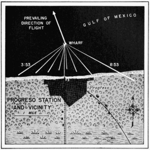
night of April 23-24, 1948, from 8:53 P. M. to 3:53 A. M. Essential features of
this map are drawn to scale. The telescope was set up on the end of a one-mile
long wharf that extends northward from the shore over the waters of the
Gulf of Mexico. The triangular (white) lines represent the projections of the
cone of visibility on the earth at the mid-point of each hour of observation.
Only briefly, in the first two hours, did the cone lie even in part over the adjacent
mainland. Hence, nearly all of the birds seen in the course of the night
had actually left the land behind.
The observation station at Progreso was situated on the northern
end of the new wharf which projects northward from the beach to
a point one mile over the Gulf. As will be seen from Figure 35, the
entire cone of observation lay at nearly all times over the intervening
ing water between the telescope on the end of the wharf and the
beach. Therefore, nearly all of the birds seen were actually observed
leaving the coast and passing out over the open waters of the
Gulf. The hourly station densities are shown in Table 7 and Figures
24 and 36. In the seventeen hours of observation on the nights of
April 23-24 and April 24-25, a total computed density of 59,200 birds
passed within one-half mile of each side of Progreso. This is the
third highest density recorded in the course of this study. The
[Pg_444]
maximum for one hour was a computed density of 11,900 birds. This
is the fourth highest hourly density recorded in 1948.
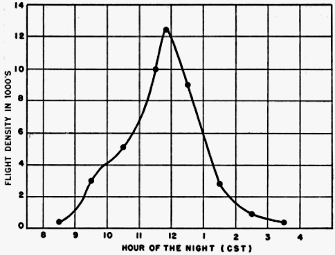
| Date | Average hour of observation | ||||||||
| 8:30 | 9:30 | 10:30 | 11:30 | 12:30 | 1:30 | 2:30 | 3:30 | 4:30 | |
| 23-24 April | 400 | 3,000 | 5,100 | 10,000 | 9,000 | 2,800 | 900 | 400 | .... |
| 24-25 April | 0 | 500 | 3,700 | 11,900 | 7,900 | 1,900 | 1,100 | 400 | 200 |
It is not my contention that this many birds leave the northern
coast of Yucatán every night in spring. Indeed, further studies may
show negligible flight densities on some nights and even greater densities
on others. As a matter of fact several hours of observation on
the night of April 25-26, at Mérida, Yucatán, approximately twenty-five
miles inland from Progreso, indicated that on this night the
density overhead was notably low, a condition possibly accounted
for by a north wind of 10 mph blowing at 2,000 feet. I merely submit
[Pg_445]
that on the nights of April 23-24 and 24-25, birds were leaving
the coast of Yucatán at Progreso at the rate indicated. But, as I
have emphasized in this paper and elsewhere (1946: 205-206), the
northern part of the Yucatán Peninsula is notably unmarked by
streams or any other physiographic features which birds might follow.
The uniformity of the topography for many miles on either
side of Progreso, if not indeed for the entire breadth of the Peninsula,
makes it probable that Progreso is not a particularly favored
spot for observing migration, and that it is not the only point along
the northern coast of Yucatán where high flight densities can be
recorded. This probability must be considered when comparisons
are made between Progreso densities and those at Tampico. The
argument could be advanced that the present densities from Tampico
do not sufficiently exceed those at Progreso to establish the
coastal route as the main avenue of traffic in spring, since there is
every reason to suspect topography of exerting some influence to
produce a channeling effect in eastern Mexico. Here the coast parallels
the directional trend of the migratory movement for more than
600 miles. Likewise the Sierra Madre Oriental of eastern Mexico,
situated approximately 100 miles inland (sometimes less), lies
roughly parallel to the coast. Because of the slant of the Mexican
land mass, many winter residents in southern Mexico, by short
northward movements, would sooner or later filter into the coastal
plain. Once birds are shunted into this lowland area, it would seem
unlikely that they would again ascend to the top of the Sierra Madre
to the west. In this way the great north-south cordillera of mountains
may act as a western barrier to the horizontal dispersion of
transients bound for eastern North America. Similarly, the Gulf
itself may serve as an eastern barrier; for, as long as migrants may
progress northward in the seasonal direction of migration and still
remain over land, I believe they would do so.
To put the matter in a slightly different way, the idea of a very
narrow flight lane is inherent in the idea of coastwise migration.
For, as soon as we begin to visualize flights of great volume over
fronts extending back more than fifty miles from the shore line, we
are approaching, if indeed we have not already passed, the point
where the phenomenon is no longer coastwise in essence, but merely
overland (as indeed my own unprocessed, telescopic data for 1949
indicate may be the case). In actuality, those who have reported on
the migration along the western edge of the Gulf of Mexico have
never estimated the width of the main flight at more than fifty miles
[Pg_446]
and have intimated that under some circumstances it may be as
narrow as two miles. No evidence of such restrictions can be discerned
in the case of the trans-Gulf flights. If it cannot be said
that they may be assumed to be as wide as the Gulf itself, they at
least have the potential breadth of the whole 260-mile northern
coast of the Yucatán Peninsula. On these premises, to be merely
equal in total magnitude, the coastwise flights must exhibit, depending
on the particular situation, from five to 130 times the concentrations
observable among trans-Gulf migrants. This point
seems almost too elementary to mention, but I have yet to find anyone
who, in comparing the two situations, takes it into consideration.
Judged in this light, the average hourly density of 2,800 birds at
Progreso in April would appear to be indicative of many more migrants
on the entire potential front than the 6,300 birds representing
the average hourly density for the same month at Tampico.
That the Progreso birds were actually beginning a trans-Gulf
flight seems inevitable. The Yucatán Peninsula projects 200 miles
or more northward into the vast open expanses of the Gulf of Mexico
and the Caribbean Sea, with wide stretches of water on either side.
The great majority of the birds were observed after they had proceeded
beyond the northern edge of this land mass. Had they later
veered either to the east or the west, they would have been obliged
to travel several hundred miles before again reaching land, almost
as far as the distance straight across the Gulf. Had they turned
southward, some individuals should have been detected flying in
that direction. As can be seen from Figures 23, 42, and 44, not one
bird observed was heading south of east or south of west on either
night. No other single piece of evidence so conclusively demonstrates
that birds cross the Gulf of Mexico in spring in considerable
numbers as do flight density data recorded from Progreso in 1948.
Unfortunately only a few data on flight density are available from
critical localities on the northern shores of the Gulf in spring. As
the density curves in Figure 30 demonstrate, several sets of observation,
including some phenomenal flights, have been recorded at
Baton Rouge. This locality, however, lies sixty-four miles from the
closest point on the Gulf coast, and the point due southward on the
coast is eighty-four miles distant. Since all of the birds seen at
Baton Rouge on any one night may have come from the heavily
forested area between Baton Rouge and the coast of the Gulf, we
cannot use data from Baton Rouge as certainly representative of
[Pg_447]
incoming trans-Gulf flights. Data from repeated observations at
stations on the coast itself are needed to judge the degree of trans-Gulf
migration northward. On the few nights of observation at
such localities (Cameron and Grand Isle, Louisiana, and Pensacola,
Florida), flight densities have been zero or negligible. To be sure,
negative results have been obtained at stations in the interior of
the United States, and flights of low density have been recorded on
occasion at stations where the flight densities are otherwise high.
Nevertheless, in view of the volume of migration departing from
Progreso, Yucatán, it would appear, upon first consideration, that
we should at times record on the coast of Louisiana enough birds
arriving in a night of continuous observation to yield a high density
figure.
Upon further consideration, however, there are factors mitigating
against heavy densities of birds in northern flight on the northern
coast of the Gulf. In the first place, presuming the main trans-Gulf
flight to originate from northern Yucatán, and that there is a directional
fanning to the northward, the birds leave on a 260-mile
front, and arrive on a front 400 miles or more wide. Consequently,
other factors remaining the same, there would be only approximately
half the number of birds on the coast of arrival, at a given
time and place, as there was on the coast of departure. Secondly,
we may now presume on the basis of the telescopic studies at Progreso,
that most migrants leaving northern Yucatán do so in the
few hours centering about midnight. The varying speeds of the
birds making the 580-mile flight across the Gulf distribute them still
more sparsely on the north coast of the Gulf both in time and in
space. Also we can see only that segment of the flight, which
arrives in that part of a twenty-four hour period when the moon
is up. This circumstance further reduces the interceptive potential
because the hours after dark, to which the present telescopic studies
have been restricted, comprise the period in which the fewest migrants
arrive from over the water. To illustrate: it is a mathematical
certainty that none of the birds leaving Yucatán in the hours
of heaviest flight, before 12 P. M., and flying on a straight course at a
speed of approximately 33 mph will reach the northern Gulf coast
after nightfall; they arrive in the daytime. It will be useful to
devise a technique for employing the sun as a background for telescopic
observation of birds, thereby making observations possible
on a twenty-four hour basis, so as to test these inferences by objective
data.
[Pg_448]
When a whole night's observation (1949 data not yet processed)
at Port Aransas, on the southern coast of Texas, on the great overland
route from eastern Mexico, yields in one night in April only
seven birds, the recording of no birds at a station near the mouth of
the Mississippi River becomes less significant.
As I have previously remarked in this paper, the new data obtained
since 1946, when I last wrote on the subject of migration in the region
of Gulf of Mexico, requires that I alter materially some of my
previously held views. As more and more facts come to light, I
may be compelled to alter them still further. For one thing, I
have come to doubt seriously the rigidity of the coastal hiatus as I
envisioned it in 1945. I believe instead that the scarcity of records
of transient migrants on the Gulf coastal plain in fair weather is to
a very large extent the result of a wide dispersion of birds in the
dense cover that characterizes this general region. I now question
if appreciable bird densities on the ground ever materialize anywhere
except when the sparseness of suitable habitat for resting
or feeding tends to concentrate birds in one place, or when certain
meteorological conditions erect a barrier in the path of an oncoming
migratory flight, precipitating many birds in one place.
This retrenchment of ideas is a direct consequence of the present
study, for time and again, as discussed in the case of Tampico densities,
maximal nightly flights have failed to produce a visible abundance
of transients on land the following day. A simple example
may serve to illustrate why. The highest one-hour density recorded
in the course of this study is 21,200 birds. That means that this
many birds crossed a line one mile long on the earth's surface and
at right angles to the direction of flight. Let us further assume that
the average flight speed of all birds comprising this flight was 30
mph. Had the entire flight descended simultaneously, it would have
been dispersed over an area one mile wide and thirty miles long,
and the precipitated density on the ground would have been only
1.1 birds per acre. Moreover, if as many as ten species had been
involved in the flight, this would have meant an average per species
of less than one bird per nine acres. This would have failed, of
course, to show appreciable concentrations to the observer in the
field the following day. If, however, on the other hand, the same
flight of 21,200 birds had encountered at one point a weather barrier,
such as a cold-front storm, all 21,200 birds might have been precipitated
in one place and the field observer would have recorded an
"inundation of migrants." This would be especially true if the
[Pg_449]
locality were one with a high percentage of open fields or prairies
and if the flight were mainly of woodland dwelling species, or conversely,
if the locality were densely forested with few open situations
and the flight consisted mainly of open-country birds. As explained
on page 389, the density formula may be too conservative in its
expression of actual bird densities. Even if the densities computed
for birds in the air are only half as high as the actual densities in the
air, the corresponding ground density of 2.2 birds per acre that
results if all the birds descended simultaneously would hardly be
any more impressive than the 1.1 bird per acre.
This consideration is doubtless highly modified by local circumstances,
but, in general, it seems to suggest a working hypothesis
that provides an explanation for many of the facts that we now
have. For example, on the coast of Texas there are great expanses
of terrain unattractive to such birds as warblers, vireos, tanagers, and
thrushes. The precipitation there by bad weather of even a mediocre
nightly flight composed of birds of the kinds mentioned would
surely produce an overwhelming concentration of birds in the
scattered woods and shrubs.
In spite of all that has been written about the great concentrations
of transient migrants on the coast of Texas in spring, I am not convinced
that they are of a different order of magnitude than those concentrations
that sometimes occur along the cheniers and coastal islands
of Louisiana and Mississippi. I have read over and over the
highly informative accounts of Professor Williams (loci cit.) and the
seasonal summaries by Davis (1936-1940) and Williams (1941-1945).
I have conversed at length with Mrs. Jack Hagar, whom I
regard as one of the leading authorities on the bird life of the
Texas coast, and she has even permitted me access to her voluminous
records covering a period of fifteen years residence at Rockport.
Finally, I have spent a limited amount of time myself on the Texas
coast studying first-hand the situation that obtains there in order
that I might be in a position to compare it with what I have learned
from observations elsewhere in the region of the Gulf of Mexico,
Louisiana, Florida, Yucatán, and eastern Mexico.
Although the concentrations of birds on some days near the mouth
of the Mississippi River are almost incalculable, the fact remains
that in Texas the densities of transient species on the ground are
more consistently high from day to day. The reason for this may
be simple. As birds move up daily from Mexico overland, a certain
percentage would be destined to come down at all points along the
[Pg_450]
route but so dispersed in the inland forest that they might pass unnoticed.
However, that part of the same flight settling down in
coastal areas, where trees are scarce, would produce visible concentrations
of woodland species. With the advent of a cold-front
storm, two diametrically opposite effects of the same meteorological
phenomenon would tend to pile up great concentrations of migrants
of two classes—the overland and the trans-Gulf flights. During the
prepolar-front weather the strong southerly (from the south) and
southeasterly winds would tend to displace much of the trans-Gulf
segment to the western part of the Gulf. With the shift of the winds
to the north and northwest, which always occurs as the front passes,
the overland flight still in the air would tend to be banked up against
the coast, and the incoming trans-Gulf flight would be confronted
with a barrier, resulting in the precipitation of birds on the first
available land.
These postulated conditions are duplicated in part in autumn
along the Atlantic coast of the eastern United States. There, as a
result of the excellent work of Allen and Peterson (1936) and Stone
(1937), a similar effect has been demonstrated when northwest
winds shove the south-bound flights up against the coast of New
Jersey and concentrate large aggregations of migrants there.
Attention has been drawn already to the nature of the nightly
flights at stations immediately inland from the Gulf coast, where
densities decline abruptly well before midnight. I have suggested
that this early drop-off is mainly a result of the small amount of
terrain south of these stations from which birds may be contributed
to a night's flight. At Oak Grove, Louisiana, the flight exhibited a
strong directional trend with no significant aberrant components.
Therefore, one may infer that a considerable part of the flight was
derived from regions to the south of the station.
At Mansfield, Louisiana, thirty-eight hours of observation in
April and May resulted in flight densities that are surprisingly low—much
lower, in fact, than at Oak Grove. In eleven of the hours
of observation no birds at all were seen. A possible explanation for
these low densities lies in the fact that eastern Texas and western
Louisiana, where, probably, the Mansfield flights originated, is not
an especially attractive region to migrants because of the great
amount of deforested and second growth pine land. Oak Grove, in
contrast, is in the great Tensas-Mississippi River flood plain, characterized
by an almost solid stand of deciduous forest extending
over thousands of square miles in the lower Mississippi valley.
[Pg_451]
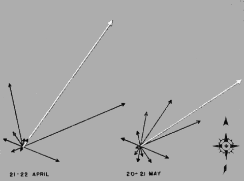
In further contrast to the considerable flight densities and pronounced
directional trend at Oak Grove, we have the results from
Rosedale, Mississippi, only seventy miles to the north and slightly
to the east. At Rosedale the densities were mediocre and the flight
directions were extremely divergent. Many of the nights of observation
at this locality were seriously interrupted by clouds, but such
counts as were made on those dates indicated little migration taking
place. On two nights, however, April 21-22 and May 20-21, visibility
was almost continuous and densities were moderately high.
In Figure 37 I have shown the flight directions for these two nights.
The lengths of the individual sector vectors are plotted as a percentage
of the total station density for each of the two nights (5,800
and 6,800 birds, respectively). Although the vector resultants show
a net movement of birds to the northeast, there are important divergent
components of the flights. This "round-the-compass" pattern
is characteristic of stations on the edge of meteorological
disturbances, as was Rosedale on April 21-22, but not on the night
of May 20-21. If bats are presumed to have played a rôle in
these latter observations, their random flights would tend to cancel
[Pg_452]
out and the vector resultant would emerge as a graphic representation
of the actual net trend density of the birds and its prevailing
direction of flow. Although I do not believe that bats are the real
reason for the diverse directional patterns at Rosedale, I can offer
no alternative explanation consistent with data from other stations.
Moving northward in the valley of the Mississippi and its tributaries,
we find a number of stations that yielded significantly high
densities on most nights when weather conditions were favorable for
migration. Louisville and Murray, Kentucky, and Knoxville, Tennessee,
each show several nights with many birds flying, but only
Lawrence, Kansas, and Ottumwa, Iowa, had migrations that approach
in magnitude the record station densities at Tampico. Indeed,
these were the only two stations in the United States that produced
flights exceeding the densities at Progreso, Yucatán. The
densities at Lawrence are unique in one respect, in that they were
extremely high in the month of March. Since there were very few
stations in operation then, these high densities would be of little
significance were it not for the fact that at no time in the course of
this study from 1945 to the present have comparable densities been
obtained this early in the migration period. Examination of the
"Remarks" section of the original data sheets from Lawrence show
frequent mention of "duck-like" birds passing before the moon.
We may infer from these notations that a considerable part of the
overhead flight was composed of ducks and other aquatic birds that
normally leave the southern United States before the main body of
transient species reach there. The heavy flight densities at Lawrence
may likewise have contained certain Fringillidae, Motacillidae,
Sylviidae, and other passerine birds that winter mainly in the
southern United States and which are known to begin their return
northward in March or even earlier. Observations in 1948 at Lawrence
in April were hindered by clouds, and in May no studies were
attempted. However, we do have at hand two excellent sets of data
recorded at Lawrence on the nights of May 3-4 and May 5-6, 1947,
when the density was also extremely high.
At Ottumwa, Iowa, where a splendid cooperative effort on the
part of the local ornithologists resulted in forty-four hours of
observation in April and May, densities were near the maximum
for all stations. Considering this fact along with results at Lawrence
and other mid-western stations where cloud cover did not
interfere at the critical periods of observation, we have here evidence
supporting the generally held thesis that eastern Kansas, Missouri,
and Iowa lie on a principal migratory flyway.
[Pg_453]
Stations in Minnesota, Illinois, Michigan, Massachusetts, and
Ontario were either operated for only parts of one or two nights, or
else clouds seriously interfered with observations, resulting in discontinuous
counts. It may be hoped that future studies will include
an adequate representation of stations in these states and that
observations will be extensive enough to permit conclusions regarding
the density and direction of migration.
Charleston, South Carolina, which does not conveniently fall in
any of the geographic regions so far discussed, had, to me, a surprisingly
low flight density; twenty-two hours of observation there
in March, April, and May yielded a total flight density of only
3,000 birds. This is less, for example, than the number of birds
computed to have passed Lawrence, Kansas, in one hour, or to have
passed Progreso, Yucatán, in one twenty-minute interval! Possibly
observations at Charleston merely chanced to fall on nights of inexplicably
low densities; further observations will be required to
clear up this uncertainty.
The belief that winds affect the migration of birds is an old one.
The extent to which winds do so, and the precise manner in which
they operate, have not until rather recently been the subject of real
investigation. With modern advances in aerodynamics and the development
of the pressure-pattern system of flying in aviation, attention
of ornithologists has been directed anew to the part that air
currents may play in the normal migrations of birds. In America,
a brief article by Bagg (1948), correlating the observed abundance
of migrants in New England with the pressure pattern obtaining at
the time, has been supplemented by the unpublished work of Winnifred
Smith. Also Landsberg (1948) has pointed out the close correspondence
between the routes of certain long-distance migrants
and prevailing wind trajectories. All of this is basis for the hypothesis
that most birds travel along definite air currents, riding with the
wind. Since the flow of the air moves clockwise around a high pressure
area and counterclockwise around a low pressure area, the birds
are directed away from the "high" and toward the center of the
"low." The arrival of birds in a particular area can be predicted
from a study of the surrounding meteorological conditions, and the
evidence in support of the hypothesis rests mainly upon the success
of these predictions in terms of observations in the field.
From some points of view, this hypothesis is an attractive one. It
explains how long distances involved in many migrations may be
[Pg_454]
accomplished with a minimum of effort. But the ways in which
winds affect migration need analysis on a broader scale than can be
made from purely local vantage points. Studies of the problem
must be implemented by data accumulated from a study of the process
in action, not merely from evidence inferred from the visible
results that follow it. Although several hundred stations operating
simultaneously would surely yield more definite results, the telescopic
observations in 1948 offer a splendid opportunity to test the
theory on a continental scale.
The approach employed has been to plot on maps sector vectors
and vector resultants that express the directional trends of migration
in the eastern United States and the Gulf region, and to compare
the data on these maps with data supplied by the U. S. Weather
Bureau regarding the directions and velocities of the winds, the location
of high and low pressure areas, the movement of cold and warm
fronts, and the disposition of isobars or lines of equal pressure. It
should be borne in mind when interpreting these vectors that they
are intended to represent the directions of flight only at the proximal
ends, or junction points, of the arrows. The tendency of the eye to
follow a vector to its distal extremity should not be allowed to create
the misapprehension that the actual flight is supposed to have continued
on in a straight line to the map location occupied by the
arrowhead.
A fundamental difficulty in the pressure-pattern theory of migration
has no doubt already suggested itself to the reader. The difficulty
to which I refer is made clear by asking two questions. How
can the birds ever get where they are going if they are dependent
upon the whim of the winds? How can pressure-pattern flying be
reconciled with the precision birds are supposed to show in returning
year after year to the same nesting area? The answer is, in
part, that, if the wind is a major controlling influence on the routes
birds follow, there must be a rather stable pattern of air currents
prevailing from year to year. Such a situation does in fact exist.
There are maps showing wind roses at 750 and 1,500 meters above
mean sea level during April and May (Stevens, 1933, figs. 13-14,
17-18). Similarly, the "Airway Meteorological Atlas for the United
States" (Anonymous, 1941) gives surface wind roses for April
(Chart 6) and upper wind roses at 500 and 1,000 meters above mean
sea level for the combined months of March, April, and May
(Charts 81 and 82). The same publication shows wind resultants
at 500 and 1,000 meters above mean sea level (Charts 108 and 109).
Further information permitting a description in general terms of
conditions prevailing in April and May is found in the "Monthly
Weather Review" covering these months (cf. Anonymous, 1948 a,
Charts 6 and 8; 1948 b, Charts 6 and 8).
[Pg_455]
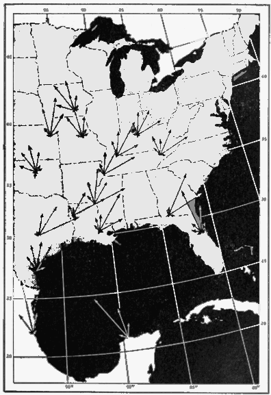
[Pg_456]
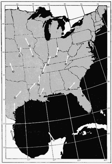
vector analysis of the over-all sector densities.
[Pg_457]
First, however, it is helpful as a starting point to consider the
over-all picture created by the flight trends computed from this
study. In Figure 38, the individual sector vectors are mapped for
the season for all stations with sufficient data. The length of each
sector vector is determined as follows: the over-all seasonal density
for the station is regarded as 100 percent, and the total for the
season of the densities in each individual sector is then expressed as
a percentage. The results show the directional spread at each station.
In Figure 39, the direction of the over-all vector resultant,
obtained from the sector vectors on the preceding map, is plotted
to show the net trend at each station.
As is evident from the latter figure, the direction of the net trend
at Progreso, Yucatán, is decidedly west of north (N 26° W). At
Tampico this trend is west of north (N 11° W), but not nearly so
much so as at Progreso. In Texas, Louisiana, Georgia, Tennessee,
and Kentucky, it is decidedly east of north. In the upper Mississippi
Valley and in the eastern part of the Great Plains, the flow
appears to be northward or slightly west of north. At Winter Park,
Florida, migration follows in general the slant of the Florida
Peninsula, but, the meager data from Thomasville, Georgia, do not
indicate a continuation of this trend.
It might appear, on the basis of the foregoing data, that birds
migrate along or parallel to the southeast-northwest extension of
the land masses of Central America and southern Mexico. This
would carry many of them west of the meridian of their ultimate
goal, obliging them to turn back eastward along the lines of net
trend in the Gulf states and beyond. This curved trajectory is undoubtedly
one of the factors—but certainly not the only factor—contributing
to the effect known as the "coastal hiatus." The question
arises as to whether this northwestward trend in the southern
part of the hemisphere is a consequence of birds following the land
masses or whether instead it is the result of some other natural
cause such as a response to prevailing winds. I am inclined to the
opinion that both factors are important. Facts pertinent to this
opinion are given below.
In April and May a high pressure area prevails over the region
of the Gulf of Mexico. As the season progresses, fewer and fewer
[Pg_458]
cold-front storms reach the Gulf area, and as a result the high
pressure area over the Gulf is more stable. Since the winds move
clockwise around a "high," this gives a general northwesterly trajectory
to the air currents in the vicinity of the Yucatán Peninsula.
In the western area of the Gulf, the movement of the air mass is
in general only slightly west of north, but in the central Gulf states
and lower Mississippi Valley the trend is on the average northeasterly.
In the eastern part of the Great Plains, however, the average
circulation veers again slightly west of north. The over-all vector
resultants of bird migration at stations in 1948, as mapped in
Figure 39, correspond closely to this general pattern.
Meteorological data are available for drawing a visual comparison
between the weather pattern and the fight pattern on individual
nights. I have plotted the directional results of four nights
of observation on the Daily Weather Maps for those dates, showing
surface conditions (Figures 40, 42, 44 and 46). Each sector vector
is drawn in proportion to its percentage of the corresponding nightly
station density; hence the vectors at each station are on an independent
scale. The vector resultants, distinguished by the large
arrowheads, are all assigned the same length, but the nightly and
average hourly station densities are tabulated in the legends under
each figure. For each map showing the directions of flight, there
is on the facing page another map showing the directions of winds
aloft at 2,000 and 4,000 feet above mean sea level on the same
date (see Figures 41-47). The maps of the wind direction show
also the velocities.
Unfortunately, since there is no way of analyzing the sector trends
in terms of the elevations of the birds involved, we have no certain
way of deciding whether to compare a given trend with the winds at
2,000, 1,000, or 0 feet. Nor do we know exactly what wind corresponds
to the average or median flight level, which would otherwise
be a good altitude at which to study the net trend or vector resultant.
Furthermore, the Daily Weather Map illustrates conditions that
obtained at 12:30 A. M. (CST); the winds aloft are based on observations
made at 10:00 P. M. (CST); and the data on birds covers in
most cases the better part of the whole night. Add to all this the fact
that the flight vectors, their resultants, and the wind representations
themselves are all approximations, and it becomes apparent that
only the roughest sort of correlations are to be expected.
However, as will be seen from a study of the accompanying maps
(Figures 40-47), the shifts in wind direction from the surface up to
4,000 feet above sea level are not pronounced in most of the instances
[Pg_459]
at issue, and such variations as do occur are usually in a
clockwise direction. All in all, except for regions where frontal
activity is occurring, the weather maps give a workable approximation
to the average meteorological conditions on a given night.
The maps (Figures 40-47) permit, first, study of the number of
instances in which the main trend of flight, as shown by the vector
resultant, parallels the direction of wind at a reasonable potential
mean flight elevation, and, second, comparison of the larger individual
sector vectors and the wind currents at any elevation below
the tenable flight ceiling—one mile.
On the whole, inspection of the trend of bird-flight and wind direction
on specific nights supports the principle that the flow of
migration is in general coincident with the flow of air. It might be
argued that when the flow of air is toward the north, and when
birds in spring are proceeding normally in that direction, no significance
can be attached to the agreement of the two trends. However,
the same coincidence of wind directions and bird flights seems to be
maintained when the wind currents deviate markedly from a northward
trajectory. Figures 46 and 47, particularly in regard to the
unusual slants of the flight vectors at Ottumwa, Knoxville, and
Memphis, illustrate that this coincidence holds even when the wind is
proceeding obliquely eastward or westward. On the night of May
22-23, when a high pressure area prevailed from southern Iowa to
the Atlantic coast, and the trajectory of the winds was northward,
migration activity at Knoxville and Ottumwa was greatly increased
and the flow of birds was again northward in the normal seasonal
direction of migration.
Further study of the data shows fairly conclusively that maximum
migration activity occurs in the regions of high barometric
pressure and that the volume of migration is either low or negligible
in regions of low pressure. The passage of a cold-front storm may
almost halt migration in spring. This was demonstrated first to me
by the telescopic method at Baton Rouge, on April 12, 1946, following
a strong cold front that pushed southeastward across the Gulf
coastal plain and over the eastern Gulf of Mexico. The winds, as
usual, shifted and became strong northerly. On this night, following
the shift of the wind, only three birds were seen in seven hours of
continuous observation. Three nights later, however, on April 15,
when the warm air of the Gulf was again flowing from the south, I
saw 104 birds through the telescope in two hours. Apropos of this
consideration in the 1948 data are the nights of May 21-22 and 22-23.
[Pg_460]
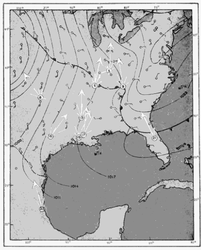
Bureau Daily Weather Map for 12:30 A. M. (CST) on April 23. The nightly
station densities and the average hourly station density (shown in parentheses)
are as follows:
|
[Pg_461]
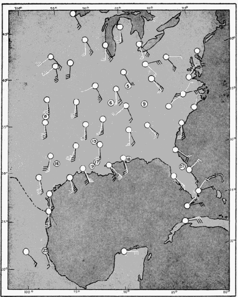
above mean sea level are shown in black; those at 4,000 feet, in white. Velocities
are indicated by standard Beaufort Scale of Wind Force. The numbers
in circles refer to the stations shown in Figure 40.
[Pg_462]
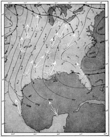
Bureau Daily Weather Map for 12:30 A. M. (CST) on April 24. The nightly
station densities and the average hourly station density (shown in parentheses)
are as follows:
|
[Pg_463]
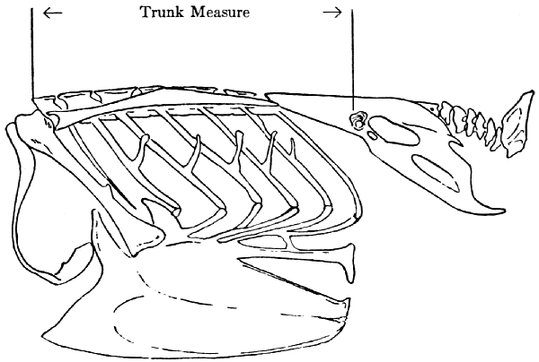
above mean sea level are shown in black; those at 4,000 feet, in white. Velocities
are indicated by standard Beaufort Scale of Wind Force. The numbers in
circles refer to the stations shown in Figure 42.
[Pg_464]
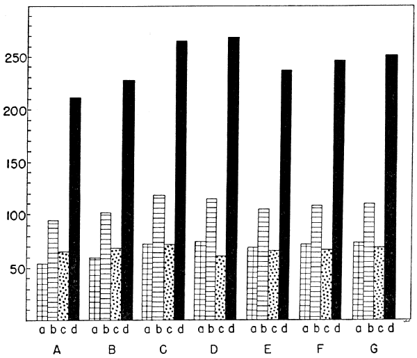
Bureau Daily Weather Map for 12:30 A. M. (CST) on April 25. The nightly
station densities and the average hourly station density (shown in parentheses)
are as follows:
|
[Pg_465]
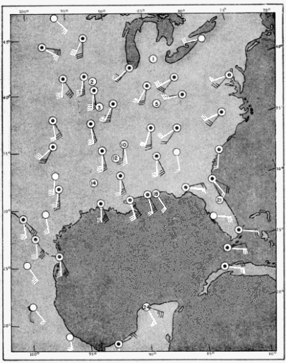
above mean sea level are shown in black; those at 4,000 feet, in white. Velocities
are indicated by standard Beaufort Scale of Wind Force. The numbers
in circles refer to the stations shown in Figure 44.
[Pg_466]
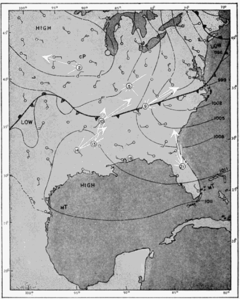
May 21-22, 1948. The meteorological data were taken from the U. S. Weather
Bureau Daily Weather Map for 12:30 A. M. (CST) on May 22. The nightly
station densities and the average hourly station density (shown in parentheses)
are as follows:
|
[Pg_467]
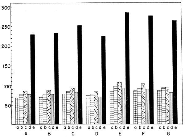
above mean sea level are shown. Velocities are indicated by standard Beaufort
Scale of Wind Force. The numbers in circles refer to the stations shown in
Figure 46.
[Pg_468]
On the first night, following the passage of a cold front, migration
at Ottumwa was comparatively low (6,900 birds in five hours). On
the following night, when the trajectory of the winds was toward the
north, the volume of migration was roughly twice as high (22,300
birds in eight hours). At Louisville, on May 21-22, the nightly
station density was only 1,500 birds in seven hours, whereas on
the following night, it was 8,400 birds in the same length of time, or
about six times greater.
The evidence adduced from the present study gives support to the
hypothesis that the continental pattern of spring migration in
eastern North America is regulated by the movement of air masses.
The clockwise circulation of warm air around an area of high pressure
provides, on its western edge, tail winds which are apparently
favorable to northward migration. High pressure areas exhibit a
centrifugal force outward from the center, which may tend to disperse
the migratory flight originating at any given point. In contrast,
the circulation of air in the vicinity of a low pressure area is
counterclockwise with the force tending to be directed inward toward
the center. Since the general movement of the air is from the high
pressure area toward a low pressure area, birds starting their migrations
with favorable tail winds, are often ultimately carried to
a region where conditions are decidedly less favorable. In the
vicinity of an area of low pressure the greater turbulence and high
wind velocities, combined with the possibly slightly less buoyant
property of the air, cause birds to descend. Since low pressure areas
in spring generally precede cold fronts, with an attending shift of
the wind to the north, an additional barrier to the northward migration
of birds is imposed. The extreme manifestation of low
pressure conditions and the manner in which they operate against
bird flight, are associated with tropical hurricanes. There, the centripetal
force of the wind is so great that it appears to draw birds
into the "eye" of the hurricane. A classic example of this effect is
seen in the case of the birds that came aboard the "West Quechee"
when this vessel passed through the "eye" of a hurricane in the Gulf
of Mexico in August, 1927. I have already discussed the details of
this incident in a previous paper (1946:192). There is also the
interesting observation of Mayhew (1949), in which a similar
observation was made of large numbers of birds aboard a ship
passing through one of these intense low-pressure areas.
Although the forces associated with an ordinary low-pressure area
are by no means as intense as those associated with a tropical hurricane,
[Pg_469]
the forces operating are much the same. Consequently birds
conceivably might tend to be drawn toward a focal point near the
center of the low, where the other factors already mentioned would
tend to precipitate the entire overhead flight. Visible evidence of
migration would then manifest itself to the field ornithologists.
| 1. | Telescopic counts of birds passing before the moon may be used to determine reliable statistical expressions of the volume of migration in terms of direction and of definite units of time and space. |
| 2. | Night migrants fly singly more often than in flocks, creating a remarkably uniform dispersion on a local scale throughout the sky, quite unlike the scattered distributions observable in the daytime. |
| 3. | The nocturnal migration of birds is apparently preceded by a resting or feeding pause during which there are few migrants in the air. It is not to an important degree a non-stop continuation of flights begun in the daylight. |
| 4. | Nightly migrational activity in North America varies from hour to hour according to a definite temporal pattern, corresponding to the Zugunruhe of caged European birds, and expressed by increasingly heavy flights up until the hour before midnight, followed by a pronounced decline. |
| 5. | The visible effects of the time pattern are subject to modification at a particular station by its location with respect to the resting areas from which the night's flight originates. |
| 6. | Quantitative and directional studies have so far failed to prove that nocturnal migrants favor narrow, topographically-determined flight lanes to an important degree. |
| 7. | Flight densities on the east coast of Mexico, though of first magnitude, have not yet been demonstrated in the volume demanded by the premise that almost all migrants returning to the United States from regions to the south do so by coastal routes. |
| 8. | Heavy flights have been recorded from the northern coast of Yucatán under circumstances leading inevitably to the conclusion that birds migrate across the Gulf of Mexico in considerable numbers. |
| 9. | There is reason to believe that the importance of the Florida Peninsula as an April and May flyway has been over-estimated, as regards the numbers of birds using it in comparison with the numbers of birds using the Mexican and Gulf routes. |
| 10. | The amount of migration is apparently seldom sufficient to produce [Pg_470] heavy densities of transient species on the ground without the operation of concentrative factors such as ecological patterns and meteorological forces. |
| 11. | The absence or scarcity of transients in some areas in fine weather may be explained by this consideration. |
| 12. | A striking correlation exists between air currents and the directional flight trends of birds, suggesting that most night migrants travel by a system of pressure-pattern flying. |
Hydrographic Office. U. S. Govt. Printing Office, Washington,
D. C., vols. 3-5.
14:65-70.
Monthly Weather Review, Supplement No. 35, November 13, pp. 1-3,
65 figs.
Vol. 1, 1-520 + 15 pp., pls. 1-46 and frontis.
Wisconsin Nat. Hist. Soc., 2:177-263.
Nat. Hist. Soc., 2:97-107.
Transmitted June 1, 1949.
23-1020
[Pg_i]
The University of Kansas Publications, Museum of Natural History,
are offered in exchange for the publications of learned societies
and institutions, universities and libraries. For exchanges and
information, address the Exchange Desk, University of Kansas
Library, Lawrence, Kansas, U. S. A.
Museum Of Natural History.—E. Raymond Hall, Chairman, Editorial Committee.
Cited as Univ. Kans. Publ., Mus. Nat. Hist.
| Vol. 1. | (Complete) Nos. 1-26. Pp. 1-638. August 15, 1946-January 20, 1951. | |
| Vol. 2. | (Complete) Mammals of Washington. By Walter W. Dalquest. Pp. 1-444, 140 figures in text. April 9, 1948. | |
| Vol. 3. | 1. | The avifauna of Micronesia, its origin, evolution, and distribution. By Rollin H. Baker. Pp. 1-359, 16 figures in text. June 12, 1951. |
| 2. | A quantitative study of the nocturnal migration of birds. By George H. Lowery, Jr. Pp. 361-472, 47 figures in text. June 29, 1951. | |
[Notes]
With the exception of the typographical corrections detailed below
and some minor corrections for missing periods or extra punctuation
(item 28 in List of Figures), the text presented here is that
contained in the original printed version. A transcription of the
Data presented in Figure 12 was added (see below) to illustrate the information
contained on that sheet. Some text was moved to rejoin paragraphs.
There are two notes in the original text indicating that the images
for Figures 41 and 45 were transposed. The correct images have been
placed with the captions and the two notes were removed. Lastly, the
cover image was compiled from a copy of the original cover with two of the
graphics contained in the article added and the list of UK pulications
was moved to the end of the document.
| Page | Correction |
| 385 | flght ⇒ flight |
| 394 | diargrams ⇒ diagrams |
| 404 | Determinaton ⇒ Determination |
| 411 | obsever ⇒ observer |
| 419 | Morover ⇒ Moreover |
| 425 | Mississippii ⇒ Mississippi |
| 425 | a ⇒ as |
| 430 | at ⇒ and |
| 431 | inserted "a" ("…traveling along a certain topographic feature…") |
| 442 | concensus ⇒ consensus |
| 472 | Stephens, Loyd A. ⇒ Stevens, Lloyd A. |
Transcription of the Data in Figure 12
|
Featured Books

Young Robin Hood
lid black; /* a thin black line border.. */ padding: 6px; /* ..spaced a bit out from the gr...
Read More
Fifty Years a Hunter and Trapper
her NotesXXVIII--The Passing of the Fur bearerXXIX--Destruction of Game and Game BirdsXXX--Southern ...
Read More
Birds and Man
artford Warbler222XIII.Vert—Vert; or Parrot Gossip249XIV.Something Pretty in a Glass Case269XV.Sel...
Read More
Birds, Illustrated by Color Photography, Vol. 1, No. 5
s among the Birds. XI. — War and Weapons among the Birds. XII. — Antics and Odor among the Bir...
Read More
Colonel Thorndyke's Secret
sidered an extraordinary crime in India, and when this occurs it becomes a religious duty for o...
Read More
The Coming of Bill
ive between the hours oftwo and four in the afternoon.The world knows little of its greatest women, ...
Read More
The Wit and Humor of America, Volume III. (of X.)
kland W. Gillilan542MaxiomsCarolyn Wells424Morris and the Honorable TimMyra Kelly488Mr. Stiver's Hor...
Read More
Jewels of Gwahlur
to test these qualities to the utmost. Ahundred and fifty feet below him waved the jungle. An equal ...
Read More
Comments on "A Quantitative Study of the Nocturnal Migration of Birds" :