The Project Gutenberg eBook of A Population Study of the Prairie Vole (Microtus ochrogaster) in Northeastern Kansas
most other parts of the world at no cost and with almost no restrictions
whatsoever. You may copy it, give it away or re-use it under the terms
of the Project Gutenberg License included with this ebook or online
at www.gutenberg.org. If you are not located in the United States,
you will have to check the laws of the country where you are located
before using this eBook.
Title: A Population Study of the Prairie Vole (Microtus ochrogaster) in Northeastern Kansas
Author: Edwin Perry Martin
Release date: April 7, 2012 [eBook #39396]
Language: English
Credits: Produced by Chris Curnow, Paula Franzini, Joseph Cooper
and the Online Distributed Proofreading Team at
https://www.pgdp.net
*** START OF THE PROJECT GUTENBERG EBOOK A POPULATION STUDY OF THE PRAIRIE VOLE (MICROTUS OCHROGASTER) IN NORTHEASTERN KANSAS ***
University of Kansas Publications
Museum of Natural History
Volume 8, No. 6, pp. 361-416, 19 figures in text
April 2, 1956
A Population Study
of the Prairie Vole (Microtus ochrogaster)
in Northeastern Kansas
BY
EDWIN P. MARTIN
University of Kansas
Lawrence
1956
University of Kansas Publications, Museum of Natural History
Editors: E. Raymond Hall, Chairman, A. Byron Leonard, Robert W. Wilson
Volume 8, No. 6, pp. 361-416, 19 figures in text
Published April 2, 1956
University of Kansas
Lawrence, Kansas
PRINTED BY
FERD VOILAND, JR., STATE PRINTER
TOPEKA, KANSAS
1956
25-9225
Contents
| PAGE | ||
| INTRODUCTION | 363 | |
| GENERAL METHODS | 364 | |
| HABITAT | 366 | |
| POPULATION STRUCTURE | 373 | |
| POPULATION DENSITY | 376 | |
| HOME RANGE | 380 | |
| LIFE HISTORY | 383 | |
| Reproduction | 383 | |
| Litter Size and Weight | 386 | |
| Size, Growth Rates and Life Spans | 388 | |
| Food Habits | 397 | |
| Runways and Nests | 398 | |
| Activity | 400 | |
| PREDATION | 401 | |
| MAMMALIAN ASSOCIATES | 403 | |
| SUMMARY AND CONCLUSIONS | 408 | |
| LITERATURE CITED | 411 | |
[363]
A POPULATION STUDY
OF THE PRAIRIE VOLE (MICROTUS OCHROGASTER)
IN NORTHEASTERN KANSAS
By
Edwin P. Martin
INTRODUCTION
Perhaps the most important species of mammal in the grasslands of
Kansas and neighboring states is the prairie vole, Microtus
ochrogaster (Wagner). Because of its abundance this vole exerts a
profound influence on the quantity and composition of the vegetation
by feeding, trampling and burrowing; also it is important in food
chains which sustain many other mammals, reptiles and birds. Although
the closely related meadow vole, M. pennsylvanicus, of the eastern
United States, has been studied both extensively and intensively,
relatively little information concerning M. ochrogaster has been
accumulated heretofore.
I acknowledge my indebtedness to Dr. Henry S. Fitch, resident
investigator on the University of Kansas Natural History Reservation.
In addition to supplying guidance and encouragement in both the
planning and execution of the investigation, Dr. Fitch made available
for study the data from his extensive field work. Interest in and
understanding of ecology were stimulated by his teaching and his
example. Special debts are also acknowledged to Mr. John Poole for the
use of his field notes and to Professor E. Raymond Hall, Chairman of
the Department of Zoology, for several courtesies. Dr. R. L. McGregor
of the Department of Botany at the University of Kansas assisted with
the identification of some of the plants. Drawings of skulls were made
by Victor Hogg.
Of the numerous publications concerning Microtus pennsylvanicus,
those of Bailey (1924), Blair (1940; 1948) and Hamilton (1937a; 1937c;
1940; 1941) were especially useful in supplying background and
suggesting methods for the present study. Publications not concerned
primarily with voles, that were especially valuable to me in providing
methods and interpretations applicable to my study, were those of
Blair (1941), Hayne (1949a; 1949b), Mohr (1943; 1947), Stickel (1946;
1948) and Summerhayes (1941). Faunal and ecological reports dealing
with M. ochrogaster and containing useful information on habits and
habitat included those of Black (1937:200-202), Brumwell
(1951:193-200; 213), Dice (1922:46) and Johnson (1926). Lantz (1907)
discussed the economic relationships of M. ochrogaster; the section
of his report concerning the effects of voles on vegetation was
especially useful to me.
Fisher (1945) studied the voles of central Missouri and obtained
information concerning food habits and nesting behavior. Jameson
(1947) studied M. ochrogaster on and near the campus of the
University of Kansas. His report is especially valuable in its
treatment of the ectoparasites of voles. In my investigation I have
concentrated on those aspects of the ecology of voles not treated at
[364]all by Fisher and Jameson, or mentioned but not adequately explored by
them. Also I have attempted to obtain larger samples.
The University of Kansas Natural History Reservation, where almost all
of the field work was done, is an area of 590 acres, comprising the
northeastern-most part of Douglas County, Kansas. Situated in the broad
ecotone between the deciduous forest and grassland, the reservation
provides a variety of habitat types (Fitch, 1952). Before 1948, much
of the area had been severely overgrazed and the original grassland
vegetation had been largely replaced by weeds. Since 1948 there has
been no grazing or cultivation. The grasses have partially recovered
and, in the summer of 1952, some grasses of the prairie climax were
present even on the parts of the Reservation which had been most
heavily overgrazed. Illustrative of the changes on the Reservation
were those observed in House Field by Henry S. Fitch (1953: in
litt.). He recalled that in July, 1948, the field supported a closely
grazed, grassy vegetation providing insufficient cover for Microtus,
with such coarse weeds as Vernonia, Verbena and Solanum
constituting a large part of the plant cover. By 1950, the same area
supported a lush stand of grass, principally Bromus inermis, and
supported many woody plants. Similar changes occurred in the other
study areas on the Reservation. Although insufficient time has elapsed
to permit analyses of successional changes, it seems that trees and
shrubs are gradually encroaching on the grassland throughout the
Reservation.
The vole population has changed radically since the Reservation was
established. In September and October of 1948, when Fitch began his
field work, he maintained lines of traps totaling more than 1000 trap
nights near the future vole study plots without capturing a single
vole. In November and December, 1948, he caught several voles near a
small pond on the Reservation and found abundant sign in the same
area. Late in 1949 he began to capture voles over the rest of the
Reservation, but not until 1950 were voles present in sufficient
numbers for convenient study.
I first visited the Reservation and searched there for sign of voles
in the summer of 1949. I found hardly any sign. In the area around the
pond mentioned above, however, several systems of runways were
discovered. This area had been protected from grazing for several
years prior to the reservation of the larger area. In House Field,
where my main study plot was to be established, there was no sign of
voles. Slightly more than a year later, in October, 1950, I began
trapping and found Microtus to be abundant on House Field and
present in smaller numbers throughout grassland areas of the
Reservation.
GENERAL METHODS
The present study was based chiefly on live-trapping as a means of
sampling a population of voles and tracing individual histories
without eliminating the animals. Live-trapping disturbs the biota less
than snap-trapping and gives a more reliable picture of the mammalian
community (Blair, 1948:396; Cockrum, 1947; Stickel, 1946:158;
1948:161). The live-traps used were modeled after the trap described
by Fitch (1950). Other types of traps were tested from time to time
but this model proved superior in being easy to set, in not springing
without a catch, in protecting the captured animal and in permitting
easy removal of the animal from the trap. A wooden box was placed
inside the metal shelter attached to each trap and, in winter, cotton
batting or woolen scraps were placed inside the boxes for nesting
material. With this insulation against the cold, voles could survive
[365]the night unharmed and could even deliver their litters successfully.
In summer the nesting material was removed but the wooden box was
retained as insulation against heat.
Bait used in live-traps was a mixture of cracked corn, milo and wheat,
purchased at a local feed store. The importance of proper baiting,
especially in winter, has been emphasized by Howard (1951) and
Llewellyn (1950) who found an adequate supply of energy-laden food,
such as corn, necessary in winter to enable small rodents to maintain
body temperature during the hours of captivity. The rare instances of
death of voles in traps in winter were associated with wet nesting
material, as these animals can survive much lower temperatures when
they are dry. Their susceptibility to wet and cold was especially
evident in rainy weather in February and March.
Preventing mortality in traps was more difficult in summer than in
winter. The traps were set in any available shade of tall grass or
weeds; or when such shade was inadequate, vegetation was pulled and
piled over the nest boxes. The traps usually were faced north so that
the attached number-ten cans, which served as shelters, cast shadows
over the hardware cloth runways during midday. Even these measures
were inadequate when the temperature reached 90°F. or above. Such high
temperatures rarely occurred early in the day, however, so that
removal of the animals from traps between eight and ten a. m. almost
eliminated mortality. Those individuals captured in the night were not
yet harmed, but it was already hot enough to reduce the activity of
the voles and prevent further captures until late afternoon. When it
was necessary to run trap lines earlier, the traps were closed in the
morning and reset in late afternoon.
Reactions of small mammals to live-traps and the effects of prebaiting
were described by Chitty and Kempson (1949). In general, the results
of my trapping program fit their conclusions. Each of my trapping
periods, consisting of seven to ten consecutive days, showed a gradual
increase in the number of captures per day for the first three days,
with a tendency for the number of captures to level off during the
remainder of the period. Leaving the traps baited and locked open for
a day or two before a trapping period tended to increase the catch
during the first few days of the period without any corresponding
increase during the latter part of the period. Initial reluctance of
the voles to enter the traps decreased as the traps became familiar
parts of their environment.
At the beginning of the study the traps were set in a grid with
intervals of 20 feet. The interval was increased to 30 feet after
three months because a larger area could thus be covered and no loss
in trapping efficiency was apparent. The traps were set within a three
foot radius of the numbered stations, and were locked and left in
position between trapping periods.
Each individual that was captured was weighed and sexed. The resulting
data were recorded in a field notebook together with the location of
the capture and other pertinent information. Newly captured voles were
marked by toe-clipping as described by Fitch (1952:32). Information
was transferred from the field notebook to a file which contained a
separate card for each individual trapped.
In the course of the program of live-trapping, many marked voles were
recaptured one or more times. Most frequently captured among the
females were number 8 (33 captures in seven months) and number 73 (30
[366]captures in eight months). Among the males, number 37 (21 captures in
six months) and number 62 (21 captures in eight months) were most
frequently taken. The mean number of captures per individual was 3.6.
For females, the mean number of captures per individual was 3.8 and
for males it was 3.4. Females seemingly acquired the habit of entering
traps more readily than did males. No correlation between any
seasonally variable factor and the number of captures per individual
was apparent. To a large degree, the formation of trap habits by voles
was an individual peculiarity.
In order to study the extent of utilization of various habitats by
Microtus, a number of areas were sampled with Museum Special
snap-traps. These traps were set in linear series approximately 25
feet apart. The number of traps used varied with the size of the area
sampled and ranged from 20 to 75. The lines were maintained for three
nights. The catch was assumed to indicate the relative abundance of
Microtus and certain other small mammals but no attempt to estimate
actual population densities from snap-trapping data was made. In
August, 1952, when the live-trapping program was concluded, the study
areas were trapped out. The efficiency of the live-trapping procedure
was emphasized by the absence of unmarked individuals among the 45
voles caught at that time.
Further details of the methods and procedures used are described in
the appropriate sections which follow.
HABITAT
Although other species of the genus Microtus, especially M.
pennsylvanicus, have been studied intensively in regard to habitat
preference (Blair, 1940:149; 1948:404-405; Bole, 1939:69; Eadie, 1953;
Gunderson, 1950:32-37; Hamilton, 1940:425-426; Hatt, 1930:521-526;
Townsend, 1935:96-101) little has been reported concerning the habitat
preferences of M. ochrogaster. Black (1937:200) reported that, in
Kansas, Microtus (mostly M. ochrogaster) preferred damp
situations. M. ochrogaster was studied in western Kansas by Brown
(1946:453) and Wooster (1935:352; 1936:396) and found to be almost
restricted to the little-bluestem association of the mixed prairie
(Albertson, 1937:522). Brumwell (1951:213), in a survey of the Fort
Leavenworth Military Reservation, found that M. ochrogaster
preferred sedge and bluegrass meadows but occurred also in a
sedge-willow association. Dice (1922:46) concluded that the presence
of green herbage, roots or tubers for use as a water source throughout
the year was a necessity for M. ochrogaster. Goodpastor and
Hoffmeister (1952:370) found M. ochrogaster to be abundant in a damp
meadow of a lake margin in Tennessee. In a study made on and near the
campus of the University of Kansas, within a few miles of the area
concerned in the present report, Jameson (1947:132) found that voles
used grassy areas in spring and summer, but that in the autumn, when
the grass began to dry, they moved to clumps of Japanese honeysuckle
(Lonicera japonica) and stayed among the shrubbery throughout the
winter. Johnson (1926:267, 270) found M. ochrogaster only in
uncultivated areas where long grass furnished adequate cover. He
stated that the entire biotic association, rather than any single
factor, was the key to the distribution of the voles. None of these
reports described an intensive study of the habitat of voles, but the
data presented indicate that voles are characteristic of grassland and
that M. ochrogaster can occupy drier areas than those used by M.
pennsylvanicus.
[367] Otherwise, the preferred habitats of the two species
seem to be much the same.
In the investigation described here I attempted to evaluate various
types of habitats on the basis of their carrying capacity at different
stages of the annual cycle and in different years. The habitats were
studied and described in terms of yield, cover and species
composition. The areas upon which live-trapping was done were studied
most intensively.
These two areas, herein designated as House Field and Quarry Field,
were both occupied by voles throughout the period of study. Population
density varied considerably, however (Fig. 5). Both of these areas
were dominated by Bromus inermis, and, in clipped samples taken in
June, 1951, this grass constituted 67 per cent of the vegetation on
House Field and 54 per cent of the vegetation on Quarry Field.
Estimates made at other times in 1950, 1951 and 1952 always confirmed
the dominance of smooth brome and approximated the above percentages.
Parts of House Field had nearly pure stands of this grass. Those traps
set in spots where there was little vegetation other than the dominant
grass caught fewer voles than traps set in spots with a more varied
cover. Poa pratensis formed an understory over most of the area
studied, especially on House Field, and attained local dominance in
shaded spots on both fields. The higher basal cover provided by the
Poa understory seemed to support a vole population larger than those
that occurred in areas lacking the bluegrass. Disturbed situations,
such as roadsides, were characterized by the dominance of Bromus
japonicus. This grass occurred also in low densities over much of the
study area among B. inermis. Other grasses present included Triodia
flava, common in House Field, but with only spotty distribution in
Quarry Field; Elymus canadensis, distributed over both areas in
spotty fashion and almost always showing evidence of use by voles and
other small mammals; Aristida oligantha and Bouteloua
curtipendula, both more common on the higher and drier Quarry Field;
Panicum virgatum, Setaria spp., especially on disturbed areas; and
three bluestems, Andropogon gerardi, A. virginicus and A.
scoparius. The bluestems increased noticeably during the study period
(even though grasses in general were being replaced by woody plants)
and they furnished a preferred habitat for voles because of their high
yield of edible foliage and relatively heavy debris which provided
shelter.
On House Field the most common forbs were Vernonia baldwini,
Verbena stricta and Solanum carolinense. On Quarry Field,
Solidago spp. and Asclepias spp. were also abundant. All of them
seemed to be used by the voles for food during the early stages of
growth, when they were tender and succulent. The fruits of the horse
nettle (Solanum carolinense) were also eaten. The forbs themselves
did not provide cover dense enough to constitute good vole habitat.
Mixed in a grass dominated association they nevertheless raised the
carrying capacity above that of a pure stand of grass. Other forbs
noted often enough to be considered common on both House Field and
Quarry Field included Carex gravida, observed frequently in House
Field and less often in Quarry Field; Amorpha canescens, more common
in Quarry Field; Tradescantia bracteata, Capsella bursapastoris,
Oxalis violacea, Euphorbia marginata, Convolvulus arvensis,
Lithospermum arvense, Teucrium canadense, Physalis longifolia,
Phytolacca americana, Plantago major, Ambrosia trifida, A.
artemisiifolia, Helianthus annuus, Cirsium altissimum and
Taraxacum erythrospermum. Both areas were being invaded from one
side by forest-edge vegetation; the woody plants noted included
[368]
Prunus americana, Rubus argutus, Rosa setigera, Cornus
drummondi, Symphoricarpus orbiculatus, Populus deltoides and
Gleditsia triacanthos.
In House Field the herbaceous vegetation was much more lush than in
Quarry Field and woody plants and weeds were more abundant. A graveled
and heavily used road along one edge of House Field, leading to the
Reservation Headquarters, was a barrier which voles rarely crossed. A
little-used dirt road crossing the trapping plot in Quarry Field
constituted a less effective barrier. The disturbed areas bordering
the roads were likewise little used and tended to reinforce the
effects of the roads as barriers. There were almost pure stands of
Bromus japonicus along both roads. No mammal of any kind was taken
in traps set where this grass was dominant.
Because seasonal changes in vole density followed the curve for rate
of growth of the complex of grasses on the Reservation, and because
years in which there was a sparse growth of plants due to dry weather
showed a decrease in the density of voles, the relationships between
productivity of plants and vole population levels on the two study
areas were investigated. In both fields the composition of the plant
cover was similar, and the differences were chiefly quantitative. In
June, 1951, ten square-meter quadrats were clipped on each of the
areas to be studied. The clippings from each were dried in the sun and
weighed. From Quarry Field the mean yield amounted to 1513 ± 302 lbs.
per acre; while from House Field the yield was 2351 ± 190 lbs. per
acre (Table 1). Using experience gained in making these samples, I
periodically estimated the relative productivity of the two areas.
House Field was from 1.5 to 3 times as productive as Quarry Field
during the growing seasons of 1951 and 1952. Although House Field,
being more productive, usually supported a larger population of voles
than Quarry Field the reverse was true at the time of the clipping
(Fig. 5).
Table 1. Relationship Between Yield and Various Population Data
| House Field | Quarry Field | |
| Yield in June, 1951, lbs./acre | 2351 ± 190 | 1513 ± 302 |
| Microtus, June, 1951, gms./acre | 3867 | 5275 |
| Per cent immature Microtus, June, 1951 | 29.85 | 38.02 |
| Ratio Microtus, June/March | 0.73 | 2.63 |
| Sigmodon, June, 1951, gms./acre | 1376 | 746 |
| Per cent immature Sigmodon, June, 1951 | 35.72 | 44.44 |
| Ratio Sigmodon, June/March | 1.40 | 2.25 |
| Microtus-Sigmodon, June, 1951, gms./acre | 5243 | 6021 |
| Microtus mean, gms./acre/month | 2922 | 1831 |
| Sigmodon mean, gms./acre/month | 802 | 335 |
| Sigmodon-Microtus, gms./acre/month | 3728 | 2166 |
Although no explanation was discovered which accounted fully for the
seeming aberration, two sets of observations were made that may bear
on the problem. In June, 1951, the population of voles and cotton rats
on Quarry Field was increasing rapidly whereas in House Field that
trend was reversed. The trends were reflected by the percentages of
immature individuals in the two populations and by the ratios of the
June, 1951, densities to the March, 1951, densities (Table 1). Perhaps
the density curve was determined in part by factors inherent in the
population and, to that extent, was fluctuating independently of the
environment (Errington, 1946:153).
The flood in 1951 reduced the population of voles and obscured the
normal seasonal trends. Although House Field produced a heavier crop
of vegetation, Quarry Field produced a larger crop of rodents, chiefly
Microtus and Sigmodon. In House Field, however, the ratio of
Sigmodon to Microtus was notably higher. Presumably the cotton
rats competed with the voles and exerted a depressing effect on their
numbers. The intensity of the effect seemed to depend on the abundance
of both species. That this depressing effect involved more than direct
competition for plant food was suggested by the fact that in House
Field, with a heavy crop of vegetation and a seemingly high carrying
capacity for both herbivorous rodents, the biomass of voles, and of
all rodents combined, were lower than in Quarry Field which had less
vegetation and fewer cotton rats. The relationships between voles and
cotton rats are discussed further later in this report.
When the centers of activity (Hayne, 1949b) of individual voles were
[369]
plotted it was seen that there was a shift in the places of high
density of voles on the trapping areas. This shift seemed to be
related to the advance of the forest edge with such woody plants as
Rhus and Symphoricarpos and young trees invading the area. These
shifts were clearly shown when the distribution of activity centers on
both areas in June, 1951, was compared with the distribution in June,
1952 (Fig. 1). The shift was gradual and the more or less steady
progress could be observed by comparing the monthly trapping records.
It was perhaps significant that during the summers the centers of
activity were less concentrated than during the winter. The shift of
voles away from the woods was more nearly evident in winter when the
voles were driven into areas of denser ground cover, which provided
better shelter.
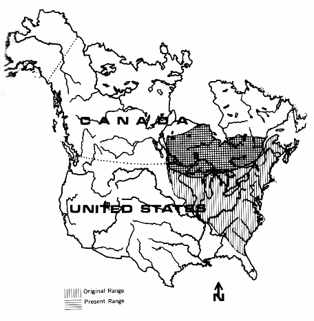
Fig. 1. Progressive encroachment of woody vegetation
onto study areas, and the accompanying shift of the centers of
populations of voles. Activity centers of individuals were calculated
as described by Hayne (1949b) and are indicated by dots. The
cross-hatched areas show places where the vegetation was influenced by
the shade of woody plants.
View larger image
From 1948 to 1950 and again in 1952 and 1953 I trapped in various
habitat types in a mixed prairie near Hays, Kansas. Before the great
drought of the thirties, Microtus ochrogaster was the most common
species of small mammal in that area. Since 1948, at least, it has
been taken only rarely and from a few habitats. No voles have been
taken from grazed sites. In a relict area, voles were trapped in a
lowland association dominated by big bluestem. Since 1948 only one
vole has been trapped in the more extensive hillside association
characterized by a mixture of big bluestem, little bluestem and
side-oats grama. None was taken in the upland parts of the relict area
where buffalo grass and blue grama dominated the association.
In the pastured areas there are nine livestock exclosures established
by the Department of Botany of Ft. Hays Kansas State College. These
exclosures included many types of habitat found in the mixed prairie.
All of these exclosures were trapped and voles were taken in only two
of them. An exclosure situated near a pond, on low ground producing a
luxuriant growth of big bluestem and western wheat grass, has
supported voles in 1948, 1949, 1952 and 1953. An upland exclosure
containing only short grasses also supported a few voles in 1953.
An examination of the nature of the various plant associations of
the mixed prairie indicates that yield of grasses, amount of debris
and basal cover may be critical factors in the distribution of voles.
The association to which the voles seemed to belong was the lowland
association. Hopkins et al (1952:401; 409) reported the yield of
grasses from the lowland to be approximately twice as great as from
the hillside and upland in most years. Probably equally important to
the voles was the fact that debris accumulation in the lowland was
[371]approximately five times as great as in the upland and approximately
2.5 times as great as on the hillside (Hopkins, unpublished data). The
unexpected presence of voles in the short grass exclosure was probably
due to two factors. In ungrazed short grass, basal cover may reach 90
per cent (Albertson, 1937:545), thus providing excellent cover for
voles. Also, the ungrazed exclosure had greater yield and a thicker
mat of debris than the grazed short grass surrounding it and was thus
a relatively good habitat, although it did not compare favorably with
the lowland type.
Samples of the populations of various areas, obtained by
snap-trapping, gave further information regarding the types of
vegetation preferred by voles. Voles were taken in all ungrazed and
unmown grasslands trapped in eastern Kansas, although some of the
areas were not used at all seasons of the year nor in years having a
low population of Microtus. Reithro Field, similar to Quarry Field
in its general aspect, had a heavy population of voles in the spring
and summer of 1951, a time when voles were generally abundant. On the
same area the population of small mammals was sampled in the summer of
1949 and, though occasional sign of voles was seen, not one vole was
trapped. Later trapping, in the spring and summer of 1952, also failed
to catch any voles and Fitch (1953, in litt.) caught none in several
trapping attempts in 1953. These later times were characterized by a
general scarcity of voles. Reithro Field was drier, with less dense
vegetation, than the two main study areas and had larger percentages
of little bluestem (Andropogon scoparius) and side-oats grama
(Bouteloua curtipendula) and smaller percentages of Vernonia,
Verbena, Solanum and Solidago.
Various species of foxtail (Setaria) dominated most roadsides in the
vicinity of the Reservation. Voles almost always used these strips of
grass but never were abundant in them. Voles were taken near the
margin of a weedy field, fallow since 1948, but there was none in the
middle of the field. Most individuals were confined to the grassy
areas around the field and made only occasional forays away from the
edge. The dam of a small pond on the Reservation and low ground near
the water were used by Microtus at all times. In the summer of 1949
no voles were taken anywhere on the Reservation but their runways were
more abundant around the pond than in the other places examined. Of
all the areas studied in the summer of 1949, only the pond area had
been protected from grazing in previous years. Polygonum coccineum
was the most prominent plant in the pond edge association. A few voles
were trapped in large openings in the woods, where a prairie
vegetation remained and where voles seemingly lived in nearly isolated
groups.
Voles were rarely taken in grazed or mown grassland or in fields of
alfalfa, stubble or row crops. The critical factor in these cases
seemed to be the absence of debris or other ground cover under which
runways and nests could be concealed satisfactorily. Woods, rocky
outcroppings and bare ground were not used regularly by voles. Fitch
(1953, in litt.) has taken several Microtus in reptile traps set
along a rocky ledge in woods but most of these voles were subadult
males and seemed to be transients. Fields in the early stages of
succession also failed to support a population of voles. Such areas on
the Reservation were characterized by giant ragweed, horse weed,
thistles and other coarse weeds. Basal cover was low and debris
scanty. Not until an understory of grasses was established did a
population of voles appear on such areas. The coarse weeds seemed to
[372]
provide neither food nor cover adequate for the needs of the voles.
An analysis of trapping success at each station in House Field further
clarified habitat preferences. The tendency of voles to avoid woody
vegetation was again demonstrated. Not only was the population
concentrated on that part of the study plot farthest from the forest
edge but, as a general rule, voles tended to avoid single trees or
clumps of shrubby plants wherever these occurred on the area. As an
example, trap number 18 never caught more than one per cent of the
monthly catch and in many trapping periods caught nothing. This trap
was under a wild plum tree. Adjacent traps often were entered; the
general area was the most heavily populated part of the study plot.
Only under the plum tree was there a relatively unused portion.
Traps number 29 and 30, in the shade of a large honey locust tree,
also caught but few voles. Trap number 30 was only six feet from the
base of the tree and caught but one vole throughout the study period.
These two traps caught more Peromyscus leucopus than any other pair,
however, and both of them also caught pine voles (M. pinetorum). The
area shaded by this tree permitted an extension of parts of the forest
edge fauna into the grassland.
In spite of the marked general tendency to avoid woody plants, some
voles made their runways around the roots of blackberry bushes, sumac
and wild plum trees. Some nests were found under larger roots, as if
placed there for protection. More vegetation was found under the woody
plants which the voles chose to use for shelter than under those which
they avoided. It seemed probable that the actual condition avoided by
voles was the bareness of the ground (a result of the shade cast by
the woody plants) rather than the woody plants themselves.
Running diagonally across the eastern half of the trapping plot in
House Field there was a terracelike ridge of soil. On each side of
this ridge there was a slight depression. Observations of the study
plot in the growing season showed this strip to produce the most
luxuriant vegetation of any part of the plot. Clip-quadrat studies
confirmed this observation and showed the bluegrass understory to be
especially heavy. This strip included the areas trapped by traps
numbered 4, 5, 17, 18, 22, 23 and 37. With the exception of trap
number 18, discussed above, these traps consistently made more
captures than traps set in other parts of the plot. In winter, these
traps also caught more harvest mice (Reithrodontomys megalotis) than
any other comparable group of traps.
Although the amount of growing tissue of plants probably is at least
as important to voles as the total amount of vegetation, some
correlation seemed to exist between the density of grassy vegetation
and the density of populations of voles. A mixed stand of grasses,
with an obvious weedy component, can support a larger population of
voles than can either a nearly pure stand of grass or the typical
early seral stages dominated by weeds. Probably the more or less
continual supply of young plants provided preferred food easily
available to voles. A more homogeneous vegetation would tend to pass
through the young and tender stage as a unit, thus causing a feast to
be followed by a relative famine.
POPULATION STRUCTURE
[373]
During the period of study the percentage of males in most of my
samples was less than 50 per cent (Fig. 2). Only once, in June, 1952,
did the mean percentage of males in samples from three areas (House
Field, Quarry Field, Fitch traps) exceed that level and then it was
only 50.1 per cent. On several occasions, however, the percentage of
males in a sample from a single area was slightly above 50 per cent.
The highest percentage of males recorded was 56.69 per cent, in a
sample taken from the Quarry Field population in June, 1952. In the
samples taken in April, 1952, the mean percentage of males was 39.67
per cent, the lowest mean recorded. The low point for one sample was
28.02 per cent in August, 1952, from Quarry Field. The mean percentage
of males in all samples taken was 45.02 ± 2.72 per cent. Percentages
observed would occur in random samples taken from a population with 50
per cent males less than one per cent of the time. Exactly 50 per cent
of the young in the 65 litters examined were classified as males but
the sample was small and the sexing of newborn individuals was
difficult.
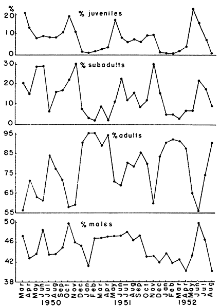
Fig. 2. Graphs of population structure showing the
monthly changes in the mean percentages of juveniles, subadults,
adults and males in samples from the three study areas.
View larger image
The extent to which sex ratios in samples were affected by trapping
procedure was not determined. A possibility considered was that the
greater wandering tendency of males (Blair, 1940:154; Hamilton,
1937c:261; Townsend, 1935:98) impaired the formation of trap habits
(Chitty and Kempson, 1949:536) on their part and thus unbalanced the
sex ratios of the samples. If this were the explanation, the apparent
sex ratio on larger areas would more nearly approximate the true
ratio, and the frequency of capture of females would exceed that of
males. The evidence is somewhat equivocal. In the populations
described here the mean number of captures per individual per month
was 2.31 for females, which was significantly greater (at the one per
cent level) than the 2.20 captures per individual per month which was
the mean number for males. This difference supports the idea that
differences in habits between the sexes result in distorted sex ratios
in samples obtained by live-trapping. Mean percentages of males did
not, however, differ significantly between the House Field-Quarry
Field samples and the samples from the Fitch trapping area, nearly
five times as large.
Three age classes, juvenal, subadult and adult, were separated on the
basis of condition of pelage. The percentage of adults in populations
varied seasonally (Fig. 2). January, February and March were the
months when the adult fraction of the population was highest and
October and November were low points, with May and June showing
percentages almost as low. The only marked variation in this seasonal
pattern occurred in July and August, 1952, when the percentage of
adults rose sharply. This was due to a depression in the reproductive
rate during the dry summer of 1952, which is discussed later in this
report. Juveniles made up only a small fraction of the population from
December through March and a relatively large fraction in the
October-November and May-June periods (Fig. 2). Again, July and August
of 1952 were exceptions to the pattern as the percentages of juveniles
in these months fell to midwinter levels. As expected, the curve of
the percentages of subadults in the population followed that of the
juveniles and preceded that of the adults. The mean percentages for
the thirty month period for which data were available were: adults,
77.72 ± 4.48 per cent; subadults, 14.06 ± 3.14 per cent; and
juveniles, 8.22 ± 2.62 per cent. Seasonal and yearly changes in the
population structure occurred, with notable variation in the ratio of
[374]
breeding females to the entire population, as discussed in this report
under the heading of reproduction.
Since some of the juveniles did not move enough to be readily
trapped, the real percentage of juveniles in the population was
probably far greater than that shown by trapping data. I tried,
[375]
therefore, to estimate the number of juveniles on the study plot each
month by multiplying the number of lactating females by the mean
litter size. As expected, the results were consistently higher than
the estimate based on trapping data. The discrepancy was largest in
April, May, June and October. During the winter there was no important
difference between the two estimates. Even when the discrepancy was
greatest, the estimated weight of the juveniles missed by trapping was
not large enough to modify the picture of habitat utilization in any
important way. I chose, therefore, to count only those juveniles
actually trapped. Although probably consistently too low, such a
figure seemed more reliable than an estimate made on any other basis.
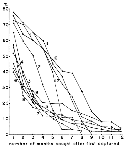
Fig. 3. Percentages of individuals captured each month
surviving in subsequent months. The graph shows differential survival
according to time of birth. Individuals born in autumn seem to have a
longer life expectancy. The numbers on the lines refer to months of
first capture.
A study of the age groups in each month's population revealed a
[376]
differential survival based on the season of birth. Blair (1948:405)
found that chances of survival in Microtus pennsylvanicus were
approximately equal throughout the year. In the present populations of
M. ochrogaster, however, voles born in October, November, December
and January tended to live longer than those born in other months
(Fig. 3). Presumably these animals, born in autumn and early winter,
were more vigorous than their older competitors and were therefore
better able to survive the shrinking habitat of winter. Their
continued survival after large numbers of younger voles had been added
to the population probably was permitted by the expanding habitat of
spring and summer. The percentage of the population surviving the
winter of 1951-1952 was approximately double the percentage surviving
the winter of 1950-1951. This difference seemed to be due to the
smaller population entering the winter of 1951-1952 rather than any
major difference in the environmental resistance.
As a consequence of the differential survival, most of the breeding
population in the spring was made up of animals born the previous
October and November. Fig. 4 shows that in February, when the
percentage of breeding females ordinarily began to rise, 51.6 per cent
of the population was born in the previous October and November. Voles
born in these two months continued to form a large part of the
population through March (45.1 per cent), April (38.5 per cent), May
(23.9 per cent), June (18.7 per cent) and July (16.2 per cent) (Fig. 4).
These percentages suggest that the habitat conditions in October
and November were probably important in determining the population
level for at least the first half of the next year.
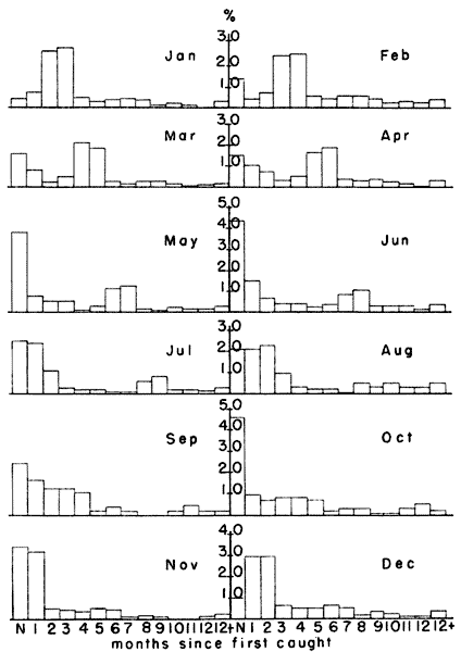
Fig. 4. Differential survival of voles according to
month when first caught. Each column represents the percentage of the
monthly sample first caught in each of the preceding months. Those
voles caught first in October and November survived longer than those
first caught in other months. Relatively few individuals remained in
the population as long as one year.
POPULATION DENSITY
Population densities were ascertained on the study areas by means of
the live-trapping program. Blair (1948:396) stated that almost all
small mammals old enough to leave the nest (except shrews and moles)
are captured by live-trapping. My experience, and that of other
workers on the Reservation, requires modification of such a statement.
The distance between traps is an important factor in determining the
efficiency of live-trapping. As mentioned earlier, when House Field
and Quarry Field were trapped out at the conclusion of the
live-trapping program no unmarked voles were taken. This showed that
the 30 foot interval between traps was short enough to cover the area
as far as Microtus was concerned. The fact that unmarked adults were
caught almost entirely in marginal traps is additional evidence. On
the other hand, the Fitch traps were 50 feet apart and voles seemed to
have lived within the grid for several months before being captured.
Fitch (1954:39) has shown that some kinds of small mammals are missed
in a live-trapping program because of variation in bait acceptance,
both seasonal and specific.
A few individuals, missed in a trapping period, were captured again
in subsequent months. These voles were assumed to have been present
during the month in which they were not caught. The area actually
trapped each month was estimated by a modification of the method
proposed by Stickel (1946:153). The average maximum move was
calculated each month and a strip one half the average maximum move in
width was added to each side of the study area actually covered by
traps. The study plots were bounded in part by gravel roads and forest
edge acting as barriers, and for these parts no marginal strip was
[377]
added. Trap lines on the opposite sides of these roads rarely caught
marked voles that had crossed in either direction. It is perhaps
advisable to say here that the size of House Field and Quarry Field
[378]study plots (0.56 acres) was too small for best results in estimating
population levels (Blair, 1941:149). In the computations of population
levels the data for males and females were combined, because no
significant difference between the average maximum move of the sexes
was apparent.
Fluctuations of the populations were graphed in terms of individuals
per acre (Fig. 5). The variation was great in the 30 month period for
which data were available, and was both chronological and
topographical. The lowest density recorded was 25.2 individuals per
acre and the highest density was 145.8 individuals per acre. The
weight varied from a low of 847 grams per acre to a high of 5275 grams
per acre.
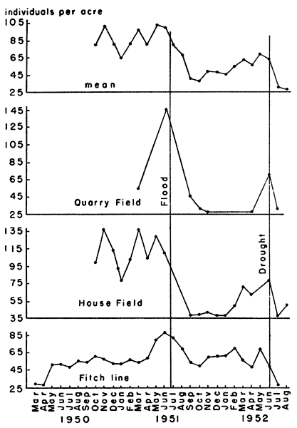
Fig. 5. Variations in density of voles from three
populations, as shown by live-trapping, and the mean density of these
populations. Juveniles are not represented in their true numbers since
many voles were caught first as subadults. The samples from the Fitch
trap line were incomplete due to the wide spacing of the traps.
There are few records of density of M. ochrogaster in the
literature. Brumwell (1951:213) found nine individuals per acre in a
prairie on the Fort Leavenworth Military Reservation and Wooster
(1939:515) reported 38.5 individuals per acre for M. o. haydeni in a
mixed prairie in west-central Kansas. High densities for M.
pennsylvanicus reported in the literature include 29.8 individuals
per acre (Blair, 1948:404), 118 individuals per acre (Bole, 1939:69),
160-230 individuals per acre (Hamilton, 1937b:781) and 67 individuals
per acre (Townsend, 1935:97).
Because the study period included one period of unusually high
rainfall and one year of unusually low rainfall, the normal pattern of
seasonal variation of population density was obscured. An examination
of the data suggested, however, that the greatest densities were
reached in October and November with a second high point in the
April-May-June period. These high points generally followed the
periods of high levels of breeding activity (Fig. 8). The autumn rise
in population may have been due, in part, to the addition of spring
and early summer litters to the breeding population, but the rise
occurred too late in the year to be explained by that alone. Another
factor may have been the spurt in growth of grasses occurring in
Kansas in early autumn, in September and October. There was a seeming
correlation between high rainfall with rapid growth of grasses and
reproductive activity, and, secondarily with high population densities
of voles. These relationships are discussed in connection with
reproduction. Lowest annual densities were found to occur in January
when there is but little breeding activity and when rainfall is low
and plant growth has ceased.
Marked deviation from the usual seasonal trends accompanied flood and
drought. In the flood of July, 1951, although the study areas were not
inundated, the ground was saturated to the extent that every footprint
at once became a puddle. Immediately after the floods, on all three
areas studied, populations were found to have been drastically
reduced. The effect was most severe on the population of House Field,
the lowest area studied, and the recovery of the population there was
much slower than that of those on the other study areas (Fig. 5).
Newborn voles were killed by the saturated condition of the ground in
which they lay. The more precocious young of Sigmodon hispidus
survived wetting better. They thus acquired an advantage in the
competitive relationship between cotton rats and voles. These
relationships are discussed more fully in the section on mammalian
associates of Microtus.
Adverse effects of heavy rainfall on populations of small mammals
have been reported by Blair (1939) and others. Goodpastor and
Hoffmeister (1952:370) reported that inundation sharply reduced
[380]
populations of M. ochrogaster for a year after flooding but that the
area was then reoccupied by a large population of voles. Such a
reoccupation may have begun on the areas of this study in the spring
of 1952 when the upward trend of the population was abruptly reversed
by drought. While cotton rats were abundant their competition may have
been an important factor in depressing population levels of voles. The
population of voles began to rise only after the population of cotton
rats had decreased (Fig. 19).
In the unusually dry summer of 1952, there was a marked decline of
population levels beginning in June and continuing to August when my
field work was terminated. Dr. Fitch (1953, in litt.) informed me
that the decline continued through the winter of 1952-53 and into the
summer of 1953, until daily catches of Microtus on the Reservation
were reduced to 2-10 per cent of the number caught on the same trap
lines in the summer of 1951. The drought seemed to affect population
levels by inhibiting reproduction, as described elsewhere in this
report. A similar sensitivity to drought was reported by Wooster
(1935:352) who found M. o. haydeni decreased more than any other
species of small mammal after the great drought of the thirties.
No evidence of cycles in M. ochrogaster was observed in this
investigation. All of the fluctuations noted were adequately explained
as resulting from the direct effects of weather or from its indirect
effect in determining the kinds and amounts of vegetation available as
food and shelter.
The differences in densities supported by the various habitats were
discussed earlier in connection with the analysis of habitats.
HOME RANGE
Home ranges were calculated for individual voles according to the
method described by Blair (1940:149-150). The term, home range, is
used as defined by Burt (1943:350-351). Only those voles captured at
least four times were used for the home range studies. Individuals
which included the edge of the trap grid in their range were excluded
unless a barrier existed (see description of habitat) confining the
seeming range to the study area.
The validity of home range calculations has been challenged (Hayne,
1950:39) and special methods of determining home range have been
advocated by a number of authors. The ranges calculated in this study
are assumed to approximate the actual areas used by individuals and
are considered useful for comparison with other ranges calculated by
similar methods, but no claim to exactness is intended. It is obvious,
for instance, that many plotted ranges contain so-called blank areas
which, at times, are not actually used by any vole (Elton, 1949:8;
Mohr, 1943:553). Studies of the movements of mammals on a more
detailed scale, perhaps by live-traps set at shorter intervals and
moved frequently, are needed to increase our understanding of home
range.
In order to test the reliability of the range calculated, an
examination of the relationship between the size of the seeming range
and the number of captures was made. For the first three months,
trapping on House Field was done with a 20 foot grid and throughout
the remainder of the study a 30 foot grid was used. The effect of
these different spacings on the size of the seeming home range was
also investigated. Hayne (1950:38) found that an increase in the
distance between traps caused an increase in the size of the seeming
[381]home range, but in my study the increased interval between traps was
not accompanied by any change in the sizes of the calculated ranges.
The number of captures, above the minimum of four, did not seem to be
a factor in determining the size of the calculated monthly range. A
seeming relationship was observed between the number of times an
individual was trapped and the total area used during the entire time
the vole was trapped. Closer examination revealed that the most
important factor was the length of time over which the vole's captures
extended. Table 2 shows the progressive increase in sizes of the mean
range of animals taken over periods of time from one month to ten
months.
Table 2. Relationship Between Home Range Size and Length of Time on
the Study Area
| No. months on area | 1 | 2 | 3 | 4 | 5 | 6 | 7 | 8 | 9 | 10 |
| Mean range in acres | .09 | .09 | .10 | .14 | .13 | .17 | .22 | .22 | .26 | .24 |
Nothing concerning the home range of Microtus ochrogaster was found
in the literature. Several workers, including Blair (1940) and
Hamilton (1937c), have studied the home range of M. pennsylvanicus.
Blair (1940:153) reported a larger range for males than for females in
all habitats and in all seasons represented in his sample. In M.
ochrogaster, however, I found that the mean monthly range for both
sexes was 0.09 of an acre. Blair (loc. cit.) reported no individuals
with a range so small as that mean, but Hamilton (op. cit.:261)
mentioned two voles with ranges of less than 1200 square feet. The
mean total range used by an individual during the entire time it was
being trapped showed a slight difference between the sexes. Males used
an average of 0.14 of an acre whereas females used an average of but
0.12 of an acre. This suggested that, as in M. pennsylvanicus
(Hamilton, loc. cit.), males tended to wander more than females and
to shift their home range more often.
The largest monthly range recorded was 0.28 of an acre used by a
female in March, 1951, and calculated on the basis of four captures.
The largest monthly range of a male was 0.25 of an acre for a vole
caught eight times in November, 1950. The smallest monthly range was
0.02 of an acre; several individuals of both sexes were restricted to
areas of this size. Juveniles, not included in the home range study,
were usually restricted to 0.01 or, at most, 0.02 of an acre. Seasonal
differences in the sizes of home ranges were not significant. However,
the voles caught in the winter often enough to be used for home range
studies were too few for a thorough study of seasonal variation in the
size of home ranges.
One female was captured 22 times in the seven-month period of
October, 1950, to April, 1951. She used an area of 0.83 of an acre,
but this actually comprised two separate ranges. From October, 1950,
through December, 1950, she was taken 17 times within an area of 0.12
of an acre; and from January, 1951, to April, 1951, she was taken five
times within an area of 0.15 of an acre. The largest area assumed to
represent one range of a female was 0.38 of an acre, recorded on the
basis of six captures in three months. The largest area encompassed by
the record of an individual male was 0.41 of an acre. He, too, shifted
his range, being taken five times on an area of 0.07 of an acre and
twice, two months later, on an area of 0.09 of an acre. Presumably,
[382]the remainder of his calculated total range was used but little, or
not at all. The largest single range of a male was 0.36 of an acre,
calculated on the basis of 18 captures in seven months. The smallest
total range for both sexes was 0.02 of an acre.
Many voles shifted their home range and a few did so abruptly. The
large range of a female vole, described above and plotted in Fig. 6,
indicated an abrupt shift from one home range to another. More common
is a gradual shift as indicated by the range of the male shown in Fig. 7.
Large parts of each monthly range of this vole overlapped the area
used in other months but his center of activity shifted from month to
month.
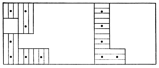
Fig. 6. Map with cross-hatched areas showing the range
of vole #20 (female). Dots show actual points of capture at permanent
trap stations 30 feet apart. Vertical lines mark area in which vole
was taken 17 times in October and November, 1950. Horizontal lines
mark area in which vole was taken five times in March and April, 1951.
This vole was not captured in December and January.
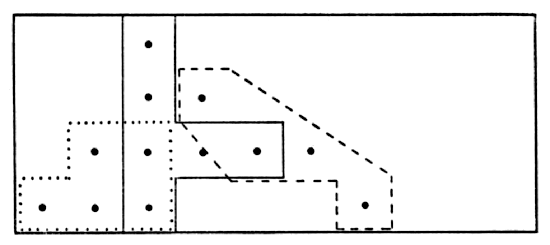
Fig. 7. Map showing range of vole #52 (male) with
seeming shifts in its center of activity. Dots show actual points of
capture at permanent trap stations 30 feet apart. Solid line encloses
points of six captures in October and November, 1950. Broken line
encloses points of five captures in February and March, 1951. Dotted
line encloses points of nine captures in April, May and June, 1951.
That home ranges overlapped was demonstrated by frequent capture of
two or more individuals together in the same trap. No territoriality
has been reported in any species of Microtus, to my knowledge, and
my voles showed no objection to sharing their range. Voles taken from
the field into the laboratory lived together in pairs or larger groups
without much friction.
[383]
Definable systems of runways and home ranges were not coextensive.
Runway systems tended to merge, as described later in this report, and
relationships between them and home range were not apparent. Home
ranges had no characteristic shape.
LIFE HISTORY
Reproduction
Reproductive activity might have been measured in a number of ways.
Three indicators were tested: the percentage of females gravid or
lactating, the percentage of juveniles in the month following the
sampling period, and the percentage of females with a vaginal orifice
in the sampling period. The condition of vagina proved to be most
useful. Whether or not there is a vaginal cycle in Microtus is
uncertain. Bodenheimer and Sulman (1946:255-256) found no evidence of
such a cycle, nor did I in my work with laboratory animals at
Lawrence. How much the artificial environment of the laboratory
affected these findings is unknown. The presence of an orifice seemed
to indicate sexual activity (Hamilton, 1941:9). The percentage of
gravid females in the population could not be determined accurately by
a live-trapping study and was not useful in this investigation. The
percentage of juveniles trapped in the month following the sampling
period tended to follow the curve of the percentage of adult females
with a vaginal orifice. The ratio of trapped juveniles to adults
trapped was a poor indicator of reproductive activity. Juveniles were
caught in relatively small numbers because of their restricted
movements, and no way to determine prenatal and juvenal mortality was
available.
Reproductive activity continues throughout the year. Within the
thirty-month period for which data were obtained, December and January
showed the lowest percentages of females with vaginal orifices (Fig. 8).
The other months all showed higher levels of reproductive activity
with a slight peak in the August-September-October period in both 1950
and 1951. In the species of Microtus that are found in the United
States, such summer peaks of breeding seem to be the rule (Blair,
1940:151; Gunderson, 1950:17; Hamilton, 1937b:785). Jameson
(1947:147) worked in the same county where my field study was made and
found that the high point of reproduction was in March, although his
samples were too small to be reliable. The peak of reproductive
activity slightly preceded the highest level of population density in
each year (Fig. 8).
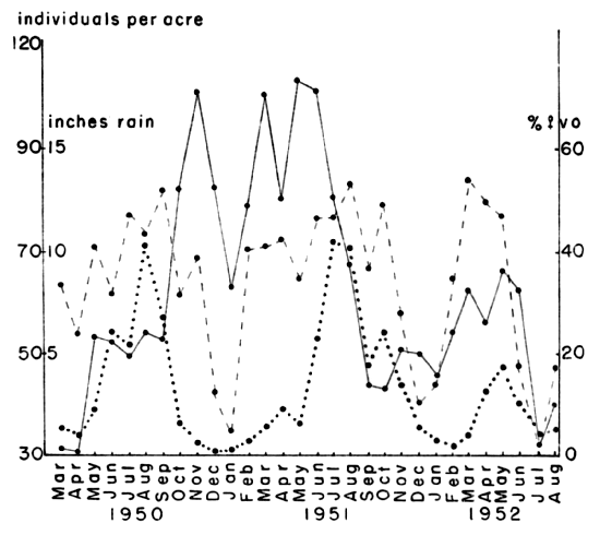
Fig. 8. Variations in density and reproductive rate of
voles, with variation in monthly precipitation. Abnormally low
rainfall in 1952 caused a decrease in breeding activity and eventually
in the numbers of voles. The solid line indicates the number of voles
per acre, the broken line the percentage of females with a vaginal
orifice and the dotted line the inches of rainfall.
A marked reduction in the percentage of females having vaginal
orifices was observed in the unusually dry summer of 1952. The rate of
reproduction was found to be positively correlated with rainfall (Fig. 9).
Correlation coefficients were higher in each case when the amount
of rainfall in the month preceding each sampling period was used
instead of that in the month of the sample. This suggested that the
rainfall exerted its influence indirectly through its effect on plant
growth. Bailey (1924:530) reported that a reduction in either the
quantity or quality of food had a depressing effect on reproduction.
Drought, such as occurred in 1952, would certainly have a depressing
effect on both. The critical factor seems to be the supply of new,
actively growing shoots available to the voles for food rather than
the total amount of vegetation. As far as could be determined from the
small sample of males examined, their fecundity was not affected by
rainfall. Some decrease in the percentage of males that were fecund
[384]
was noted in the winter and was reported also by Jameson (1947:145)
but most of the males in any sample were fecund. Thus any depression
in the reproductive rate was due to loss of fecundity by females. This
was in agreement with reports in the literature on the subject (Baker
and Ransom, 1932a:320; 1932b:43).
The correlation coefficient between rainfall and the percentage of
adult females with a vaginal orifice was 0.53. This was considered to
be surprisingly high in view of the expected effects on the breeding
rate of temperature, seasonal diet variations and whatever rhythms
were inherent in the voles. When only the summer months were
considered the correlation coefficient between rainfall and the
percentage of adult females with a vaginal orifice was 0.84. This
indicated that, during the season when breeding was at its height,
rainfall was a factor in determining the rate of reproduction and when
rainfall was scarce, as in the summer of 1952, it seemed to be a
limiting factor (Fig. 9).
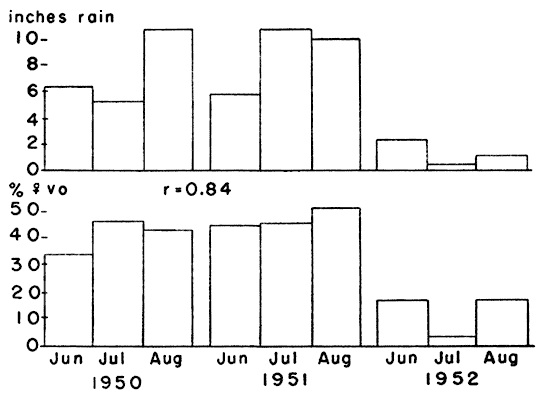
Fig. 9. Comparison between monthly rainfall and
reproductive rate of voles in summer. The dry summer of 1952 caused a
notable decrease in reproductive activity. The correlation coefficient
between rainfall and the percentage of females with a vaginal orifice
was 0.84.
Of the total captures 20.6 per cent involved more than one
individual. When the distribution of these multiple captures was
[385]
graphed for the period of study, a high correlation between the
percentage of captures that were multiple and the percentage of
females with a vaginal orifice (r = 0.70) was found. An even higher
correlation (r = 0.76) was observed between the percentage of captures
that were multiple and the population density. The higher percentage
of multiple captures may have been largely a result of fewer available
traps per individual on the area and thus only indirectly related to
the rate of reproduction.
Of the multiple captures, 66 per cent involved both sexes. The
correlation coefficient between the percentage of captures involving
both sexes and the level of reproductive activity was 0.58. Among
those pairs of individuals caught together more than once, 61 per cent
were composed of both sexes. Among those pairs taken together three or
more times 76 per cent were male and female and among those pairs
taken together four or more times 80 per cent were male and female.
When adult voles stayed together any length of time their relationship
usually appeared to be connected with sex. Family groups were also
noted, as pairs were often trapped which seemed to be mother and
offspring. A lactating female would sometimes enter a trap even after
it had been sprung by a juvenile, presumably her offspring, or a
juvenal vole would enter a trap after its mother had been captured.
Such family groups persisted only until the young voles had been
weaned.
[386]
The youngest female known to be gravid was 26 days old and weighed 28
grams. During summer most of the females were gravid before they were
six weeks old, although females born in October and after were often
more than 15 weeks old before they became gravid. The youngest male
known to be fecund was approximately six weeks old. Male fecundity was
determined as described by Jameson (1950). Difference in the age of
attainment of sexual maturity serves to reduce the mating of litter
mates (Hamilton, 1941:7) and has been noticed in various species of
the genus Microtus by several authors (Bailey, 1924:529; Hatfield,
1935:264; Hamilton, loc. cit.; Leslie and Ransom, 1940:32).
For 35 females, each of which was caught at least once each month for
ten consecutive months or longer, the mean number of litters per year
was 4.07. Certain of the more productive members of the group produced
11 litters in 16 months. M. ochrogaster seems to be less prolific
than M. pennsylvanicus. Bailey (1924:528) reported that one female
meadow vole delivered 17 litters in 12 months. Hamilton (1941:14)
considered 17 litters per year to be the maximum and stated that in
years when the vole population was low the females produced an average
of five to six litters per year. In "mouse years" the average rose to
eight to ten litters per year. During this study several females
delivered two or more litters in rapid succession. This was noted more
frequently in spring and early summer than in other parts of the year.
Those females which produced two or three litters in rapid succession
in spring and early summer often did not litter again until fall.
Post-parous copulation has been observed in M. pennsylvanicus by
Bailey (1924:528) and Hamilton (1940:429; 1949:259) and probably
occurs also in M. ochrogaster.
The gestation period was approximately 21 days, the same as reported
for M. pennsylvanicus (Bailey, loc. cit.; Hamilton, 1941:13) and
M. californicus (Hatfield, 1935:264). A more precise study of the
breeding habits of M. ochrogaster failed to materialize when the
voles refused to breed in captivity. Fisher (1945:437) also reported
that M. ochrogaster failed to breed in captivity although M.
pennsylvanicus (Bailey, 1924) and M. californicus (Hatfield, 1935)
reproduced readily in the laboratory.
Litter Size and Weight
In the course of this study 65 litters were observed. The mean number
of young per litter was 3.18 ± 0.24 and the median was three (Fig. 10).
Three litters contained but one individual and the largest litter
contained six individuals. Other investigators have reported the
number of young per litter in M. ochrogaster as three or four
(Lantz, 1907:18) and 3.4 (1-7) (Jameson, 1947:146). M.
pennsylvanicus seems to have larger litters. Although Poiley
(1949:317) found the mean size of 416 litters to be only 3.72 ± 0.18,
both Bailey (1924:528) and Hamilton (1941:15) found five to be the
commonest number of young per litter in that species. Leslie and
Ransom (1940:29) reported the average number of live births per litter
to be 3.61 in the British vole, M. agrestis. Selle (1928:96)
reported the average size of five litters of M. californicus to be
4.8. Hatfield (1935:265), working with the same species, found that
litter size varied directly with the age of the female producing the
litter. He reported litters of young females as two to four young per
litter and of older females as five to seven young per litter. In the
[387]litters of M. ochrogaster that I examined, young females did not
have more than three young and usually had but two. However, older
females had litters of one, two and three often enough so that no
relationship, as described above, was indicated clearly.

Fig. 10. Distribution of litter size among 65 litters
of voles.
No seasonal variation in litter size was noted. The mean size of the
litters in 1950, 2.68 ± 0.30, was significantly lower than that found
in 1951 (3.76 ± 0.20) but neither differed significantly from the mean
size of litters in 1952 (3.35 ± 0.66). The lower mean size of litters
was in part coincidental with a high population level and the higher
mean of the two later years was in part coincidental with a low
population level. Since a sharp break in the curve for population
density occurred after the flood in July, 1951, the litters were
arranged in pre-flood and post-flood categories for study. Pre-flood
litters averaged 3.07 ± 0.28 young per litter whereas post-flood
litters averaged 3.34 ± 0.48. This difference was not significant.
Increase in litter size, if it had actually occurred, might have been
a response to the increasing food supply and lower population density
after the flood.
A difference in the mean number of young per litter was noted for
those litters delivered in traps as compared with those delivered in
captivity and the numbers of embryos examined in the uterus. The mean
number of embryos per female was higher than the mean number of young
per litter delivered in captivity and the mean number of young per
litter delivered in traps was lower than in those delivered in
captivity. The differences were not statistically significant. In some
instances females that delivered young voles in traps may have
delivered others prior to entering the trap or the mother or her
trapmates may have eaten some of the newborn voles before they were
discovered.
[388]
The mean weight of 16 newborn (less than one day old) individuals was
2.8 ± 0.36 grams. No other data on the weight of newborn M.
ochrogaster were found in the literature but this mean was close to
the 3.0 grams (Bailey, 1924:530) and 2.07 grams (Hamilton, 1937a:504;
1941:10) reported for M. pennsylvanicus and to the 2.7 grams (Selle,
1928:97) and 2.8 grams (Hatfield, 1935:268) reported for M.
californicus. No correlation between the weight of the individual
newborn vole and the number of voles per litter was observed.
Although the ratio of the average weight of newborn voles to the
average weight of an adult female was approximately equal for M.
pennsylvanicus and M. ochrogaster, the ratio of the weight of a
litter to the average weight of an adult female was larger in the
eastern meadow vole because the mean litter size was larger. Perhaps
this is related to the more productive habitat in which the eastern
meadow vole is ordinarily found.
Size, Growth Rates and Life Spans
The mean weight of adult voles during the period of study was 43.78
grams. The females averaged slightly heavier than the males but the
overlapping of weights was so extensive that sexual difference in
weight could not be affirmed. The difference observed was less in
December and January when gravid females were rare, suggesting that
the difference was due, at least in part, to pregnancy. Jameson
(1947:128) found, for a sample of 50 voles, a mean weight of 44 grams
and a range of 38 to 58 grams. The range in the adult voles I studied
was much greater, from 25 to 73 grams. In part, this increase in the
range of adult weights was due to a much larger sample.

Fig. 11. Relationship between rainfall and the
mean weight of adult males
in summer. The abnormally low rainfall in the
summer of 1952 was accompanied by a decrease in mean weight. The solid
line represents mean weight and the broken line rainfall. The
correlation coefficient between the two was 0.68.
During the unusually dry summer of 1952, a notable reduction in the
mean weight of adults was recorded (Fig. 11). The correlation
coefficient between the mean weight of adults and the amount of
rainfall for the summer months was 0.68. It seems reasonable to
[389]attribute the drop in mean weight to an alteration of plant growth due
to decreased rainfall. Some of the reduction in mean weight was due to
the loss of weight in older individuals but most of it was due to the
failure of voles born in the spring to continue growing.
No data on the growth rate of M. ochrogaster were found in the
literature. According to the somewhat scanty data from my study,
secured from observations of individuals born in the laboratory, young
voles gained approximately 0.6 of a gram per day for the first ten
days, approximately one gram per day up to an age of one month, and
approximately 0.5 of a gram per day from an age of one month until
growth ceases. This growth rate was especially variable after the
voles reached an age of thirty days. The growth rate approximates
those described for M. pennsylvanicus (Hamilton, 1941:12) and for
M. californicus (Hatfield, 1935:269; Selle, 1928:97). Although the
data were inadequate for a definite statement, I gained the impression
that there was no difference between the sexes in growth rate. In
general, young voles grow most rapidly in the April-May-June period
and least rapidly in mid-winter. Several voles, born in late autumn,
stopped growing while still far short of adult size and lived through
the winter without gaining weight, then gained as much as 30 per cent
after spring arrived (Fig. 12).

Fig. 12. Growth rates of two voles selected to show
typical growth pattern of voles born late in the year. Growth nearly
stops in winter and is resumed in spring.
The recorded life spans of most voles studied were less than one
year. No accurate mean life span could be determined. Leslie and
Ransom (1940:46), Hamilton (1937a:506) and Fisher (1945:436) also
found that most voles lived less than one year. Leslie and Ransom
(op. cit.: 47) reported a mean life span of 237.59 ± 10.884 days in
voles of a laboratory population. In the present study one female was
trapped 624 days after first being captured; another female was
trapped 617 days after first being captured; and a male was trapped
611 days after first being captured. The two females were subadults
[390]when first captured. The male was already an adult when first
captured; consequently its life span must have exceeded 650 days. No
evidence of any decrease in vigor or fertility was observed to
accompany old age.
Of the 45 marked voles snap-trapped in August of 1952, 21 had been
captured first as juveniles. The ages of these voles could be
estimated within a few days, and the series presented a unique
opportunity for studying individual and age variation. Only
individuals weighing less than 18 grams when first captured were used,
and their ages were estimated according to the growth rate described
above. Howell (1924) reported an analysis of individual and age
variation in a series of specimens of Microtus montanus, and Hall
(1926) studied the changes due to growth in skulls of Otospermophilus
grammarus beecheyi. The series of specimens described here differs
from those of Hall and Howell, and from any other collection known to
me, in the fact that the specimens are of approximately known age and
drawn from a wild population.
Unfortunately, this sample was small, and the distribution of the
specimens among age groups left much to be desired. No specimens less
than one and one-half months old were taken and only a few individuals
older than four and one-half months. Table 3 shows the age
distribution. The small size of the sample and the absence of
juveniles were due, partly, to the unusually dry weather in the summer
of 1952. The reduction in the rate of reproduction, caused by drought
(as described elsewhere in this paper), reduced the populations and
the percentage of juveniles to low levels.
Table 3. Distribution Among Age Groups of 21 Voles Used in the Study
of Variation Due to Age
| Age in months | 11⁄2 | 2 | 21⁄2 | 3 | 31⁄2 | 4 | 41⁄2 | 6 | 12 |
| No. of individuals | 1 | 4 | 5 | 1 | 3 | 2 | 3 | 1 | 1 |
In the series of voles studied, ten individuals were in the process of
molting from subadult to adult pelage. Jameson (1947:131) reported the
molt to occur between eight and 12 weeks of age and selected 38 grams
as the lower limit of weight of adults. I also found all voles molting
to be between eight and 12 weeks old but found none so large as 38
grams without full adult pelage. This may have been, in part, due to
the dry weather delaying or inhibiting growth. Because of the small
size of the sample and the influence of the unusual weather
conditions, no conclusions concerning normal molting were drawn from
the data described below. They are presented only as a description of
a small sample drawn from a single population at one time. Table 4
summarizes these data.
Table 4. Mean Sizes and Ages of Voles Molting from Subadult to Adult
Pelage
| Weight | Body length minus tail | Condylo-basilar length | Age | |
| Six males | 32.67 gms. | 106.16 mm. | 23.78 mm. | 9.67 wks. |
| (30-36) | (96-116) | (23.2-24.4) | (8-12) | |
| Four females | 29.0 gms. | 100.25 mm. | 23.45 mm. | 10.5 wks. |
| (28-30) | (98-102) | (23.5-23.8) | (8-12) | |
| Ten voles | 31.2 gms. | 103.8 mm. | 23.73 mm. | 10.0 wks. |
| (28-36) | (96-116) | (23.2-24.4) | (8-12) |
The mean age of the ten voles molting was ten weeks (8-12). Six males
[396]
averaged 9.67 weeks, almost a week younger than four females, who
averaged 10.5 weeks. The difference in age at time of molting between
the sexes was not significant. Differences between the sexes in other
characteristics to be described also lacked significance. Mean weights
at the time of molting were: males, 32.67 gms. (30-36); females, 29.0
gms. (28-30); and all individuals, 31.2 gms. (28-36). Because a piece
of the tail of each vole had been removed in marking, the total length
of the voles could not be determined. Body length, excluding tail, was
used. Howell (1924:986) found this measurement subject to less
individual variation than total length and thought body length was
probably a better indicator of age. Mean body length at the time of
molting was 103.8 mm. (96-116). Males averaged longer than females and
were also more variable. The mean body length of males was 106.16 mm.
(96-116) and that of females was 100.25 mm. (98-102).
Of the subadults showing no signs of molting, none was above the mean
age of molting. Twenty-five per cent of them were longer and heavier
than the mean length and weight of those that were molting. Of the 20
adults in the series, one was below the mean weight of molting and one
was shorter than the mean length of molting.
When Howell (op. cit.:1014) studied skulls of Microtus montanus he
found that the condylobasilar length was the most satisfactory means
for arranging his series of specimens according to their age. When the
skulls of my series were arranged according to their age (as
determined from trapping records) the graph of the condylobasilar
lengths showed a clear, though not perfect, relationship to age (Fig. 13). No separation of sexes was made because the sample did not permit
it. In Fig. 13 graphs of weight, as determined in the field, and of
length (excluding tail) also were included because they are the most
easily measured characters of live voles. The graphs indicate
individual variation in these characters which limits their usefulness
in determining age.

Fig. 13. Graphs of the condylobasilar lengths, body
lengths and weights of a series of voles of known age. Within each age
group, the youngest vole is on the left in the graphs.
When other cranial measurements, and ratios of pairs of measurements,
were plotted in the same order, individual variation obscured some of
the variation due to age and the curves resembled those of weight and
length of body rather than that of condylobasilar length. When the
cranial measurements were averaged for the age groups the curves
showed a relationship to age but the relationship of mean measurements
is of little use in determining the age of individual specimens. The
data described above indicated that a study of the relationship of the
condylobasilar length and age in a large sample might provide useful
information.
Anyone who has examined mammalian skulls knows of many other
characters which vary with age but which are difficult to measure and
describe with precision. Figs 14 and 15 are drawings of skulls of
voles of known age. The most obvious change, related to aging, evident
in the dorsal view of the skulls (Fig. 14) is the increasing
prominence and closer approximation of the temporal ridges in older
specimens. The lambdoidal ridge is also more prominent in older voles,
and their skulls have a generally rougher and more angular appearance.
The individual variation evident in these ridges is probably due to
variations in the development of the muscles operating the jaws
(Howell, 1924:1003). There is an increased flattening of the roof of
the skull of older voles.

Fig. 14. Dorsal views of skulls of voles of known age.
(Ages 11⁄2, 21⁄2, 3, 31⁄2, 4, 41⁄2, 6 and 12 months). All × 3.
View larger image

Fig. 15. Palatal views of skulls of voles of known age.
(Ages 11⁄2, 21⁄2, 3, 31⁄2, 4, 41⁄2, 6 and 12 months). All × 3.
View larger image
From a palatal view (Fig. 15) the skulls of voles also showed age
[397]
variation which was apparent but not easily correlated with precise
age. The median ridge on the basioccipital bone increases in
prominence in older voles. The shape of the posterior margin of the
palatine bones changes from a V-shape to a U-shape. On the skull of
the oldest (12 months) vole the pterygoid processes are firmly fused
to the bullae, a condition not found in any of the other specimens.
The anterior spine of the palatine approaches the posterior projection
of the premaxillae more closely as age increases and, in the oldest
vole is firmly attached and forms a complete partition separating the
incisive foramina.
Tooth wear during the life of a vole causes a considerable variation
in the enamel patterns, especially of the third upper molar. Howell
(1924:1012) considered such variation to be independent of age, but
Hinton (1926:103) related the changes to age and interpreted them as a
recapitulation of the evolution of microtine molars. In my series, an
indentation on the medial margin of the posterior loop of the third
upper molar seemed to be related to age. This indentation was absent
in the youngest vole (one and one-half months), absent or indefinite
in those voles less than 31⁄2 months of age, and progressively more
marked in the older voles.
Food Habits
The prairie vole, like other members of the genus Microtus, feeds
mostly on growing grass in spring and summer. Piles of cuttings in the
runways are characteristic sign of the presence of voles. The voles
cut successive sections from the bases of grasses until the young and
tender growing tips are within reach. The quantity of grass destroyed
is greater than that actually eaten, a fact which will have to be
considered in any attempt to evaluate the effects of voles upon a
range.
In all piles of cut plants that were examined, Bromus inermis was
the most common grass, and Poa pratensis was the grass second in
abundance. These were, by far, the most common grasses present on the
areas studied; in most places, B. inermis was dominant. Other
grasses present on the areas were occasionally found in the piles of
cuttings. Jameson (1947:133-136) found no utilization of B. inermis
by voles but that grass was present in a relative abundance of only
one per cent in the areas studied by him. The voles that he studied
ate alfalfa in large amounts and alfalfa was, perhaps, the most common
plant on the particular areas where his voles were caught. Seemingly,
the diet of voles is determined mostly by the species composition of
the habitat.
Other summer foods included pokeberries, blackberries and a few forbs
and insects. Forbs most commonly found in the piles of cuttings were
the leaves of the giant ragweed (younger plants only) and dandelion.
Insect remains were found in the stomachs of voles killed in summer
and occurred most frequently in those killed in August and September.
At no time did insects seem to be a major part of the diet but they
were present in most vole stomachs examined in late summer. Laboratory
experiments with summer foods gave inconclusive results but suggested
that the voles chose grasses on the basis of their growth stage rather
than according to their species. Young and tender grasses were chosen,
regardless of species, when various combinations of Triodia flava,
Bromus inermis and Poa pratensis were offered to the voles. At
[398]
times the voles showed a marked preference for dandelion greens,
perhaps because of their high moisture content; the voles' water needs
were satisfied mostly by eating such succulent vegetation.
Winter foods consisted of stored hay and fruits and of underground
plant parts. Bromus inermis made up nearly all of the hay and was
stored in lengths of up to ten inches in underground chambers
specially constructed for storage. Underground parts of plants were
reached by tunnelling and were an especially important part of the
voles' diet in January and February. The fruit of Solanum
carolinense was eaten throughout the winter and one underground
chamber, opened in February, 1952, was packed full of these seemingly
unsavory fruits. Fisher (1945:436), in Missouri, found this fruit to
be an important part of the winter diet of voles. An occasional pod of
the honey locust tree was found partly eaten in a runway. Fitch (1953,
in litt.) often observed girdling of honey locust and crab apple
(Pyrus ioensis) root crowns on the Reservation but I saw no evidence
of bark eating, perhaps because my study plots were mostly grassland.
On two occasions when two voles were in the same trap one of them was
eaten. In both traps, all of the bait had been eaten and the captured
voles probably were approaching starvation. Because the trapping
procedure offered abundant opportunity for cannibalism, the low
frequency of its occurrence suggested that it was not an important
factor in satisfying food requirements under normal conditions.
Runways and Nests
Perhaps the most characteristic sign of the presence of Microtus
ochrogaster were their surface runways and underground tunnels. Only
rarely was a vole observed to expose itself to full view. When a
trapped vole was released it immediately dove out of sight into a
runway. Once in a runway, the vole showed no further evidence of alarm
and was usually in no hurry to get away. The runways seemed to provide
a sense of security and the voles were familiar with their range only
through runway travel. The urge to seek a runway immediately when
exposed has obvious survival value.
Surface runways were usually under a mat of debris. In areas where
debris was scanty or lacking, runways were usually absent. Jameson
(1947:136) reported that in alfalfa and clover fields the voles did
not make runways as they did in grassland, even in fields where
trapping records showed voles to be abundant. Typical surface runways
are approximately 50 mm. wide, only slightly cut into the ground and
bare of vegetation while in use. Usually they could be distinguished
from the runways of the pine vole, which were cut more deeply into the
ground, and those of the cotton rat which were wider and not so well
cleared of vegetation. Some runways ended in surface chambers and some
of these were lined with grass. Their size varied from a diameter of
90 mm. to 250 mm. and they seemed to be used primarily for resting
places.
A runway system usually consisted of a long, crooked runway and
several branches. Two typical systems are illustrated in Fig. 16. The
runway systems often were not clearly limited; they merged with other
systems more or less completely. One map showed a runway system
extending across 140 square meters and including 12 underground
burrows. All of these runways seemed to be part of a single runway
system but the system probably was used by more than one vole or
family group of voles. Sixteen of the 22 maps that were made extended
[399]across areas between 50 and 90 square meters. One map, mentioned
above, was larger and the remaining five smaller. The smallest
extended across only 20 square meters. Of course, the area encompassed
by a set of runways changed almost daily, as the voles extended some
runways, added some and abandoned others in the course of their daily
travels.

Fig. 16. Maps of runway systems of the prairie vole.
The runways follow an irregular course and are frequently changed. The
solid lines represent surface runways and the dotted lines underground
passages.
[400]
Each runway system contained underground nests. These were in chambers
from 70 mm. to 200 mm. below the surface and were up to 200 mm. in
diameter. Most systems that were mapped had from two to six of these
burrows. Most of these were lined with dried grass and seemed to be
used for delivering and nursing litters. Each burrow was connected to
a surface runway by a tunnel. Often the tunnel was short and the hole
opened almost directly into the burrow from the surface runway. Others
had tunnels several meters long. Jameson (1947:137) reported every
burrow to have two connections with the surface. In the present study,
however, I found three arrangements in approximately equal frequency
of occurrence: (1) one hole to one tunnel leading to a burrow; (2) two
holes to two short tunnels which joined a long tunnel leading to a
burrow; and (3) two separate tunnels from the surface to a burrow. The
size, depth and number of underground burrows in the systems that I
studied varied and so did those reported in the literature. Jameson
(loc. cit.) found burrows in eastern Kansas as deep as 18 inches,
far deeper than any found in my study. Fisher (1945:435) reported none
deeper than five inches in central Missouri. The soil data in my
study, as well as in the two reports cited immediately above, were not
adequate to permit conclusions, but the type and condition of the soil
probably determine the extent of burrowing by the voles of any given
locality.
The number of voles using a runway system at one time was difficult to
ascertain. In one system, however, four adult individuals were trapped
in a ten day period. In August, 1952, at the conclusion of the
live-trapping program, a runway system was mapped which had included
two trapping stations. In the preceding ten days, four adult voles
(three males and one female) had been taken in both traps. During that
time, therefore, the runway system was shared by at least four voles.
The voles used an area that was considerably larger than that
encompassed by any one runway system, a fact obvious when the sizes of
home ranges as computed from trapping data were compared with the
sizes of the runway systems mapped. A runway system seemed not to be a
complete unit, but was only a part of the network of runways used by a
single individual.
Activity
Although no special investigation of activity was made, some
conclusions concerning it were apparent in the data gathered. There
have been a few laboratory studies of the activity pattern of
Microtus by various methods. Calhoun (1945:256) reported M.
ochrogaster to be mainly nocturnal with activity reaching a peak
between dark and midnight and again just before dawn. Davis
(1933:235), working with M. agrestis, and Hatfield (1935:263),
working with M. californicus, both found voles to be more nocturnal
than diurnal. In a field study of M. pennsylvanicus, Hatt (1930:534)
found the species to be chiefly nocturnal, although some activity was
reported throughout the day. Hamilton (1937c:256-259), however,
reported the same species to be more active in the daytime. Agreement
on the activity patterns of these species of Microtus has not yet
been attained.
From occasional changes in the time of tending a trap line, and from
running lines of traps at night a few times in the summer of 1951, I
gained the impression that these voles were primarily diurnal.
Relatively few of them were caught in the hours of darkness. In
summer, however, their activity
[401]
was mostly limited to the periods
between dawn and approximately eight o'clock and between sunset and
dark. In colder weather, there was increased activity on sunny days.
PREDATION
Although voles were a common item of prey for many species of
predators on the Reservation, no marked effect on the density of the
population of this vole could be attributed to predation pressure.
Only when densities reached a point that caused many voles to expose
themselves abnormally could they be heavily preyed upon. Their
normally secretive habits, keeping them more or less out of sight,
suggest that they are an especially obvious illustration of the
concept that predation is an expression of population vulnerability,
rising to high levels only when a population is ecologically insecure,
rather than a major factor regulating population levels (Errington,
1935; 1936; 1943; Errington et al, 1940).
Scats from predatory mammals and reptiles and pellets from raptorial
birds were examined. Most of these materials were collected by Dr.
Henry S. Fitch, who kindly granted permission to use them. The results
of the study of the scats and pellets are summarized in Table 5.
Remains of voles were identified in 28 per cent of the scats of the
copperhead snake (Ancistrodon contortix) examined. Copperheads were
moderately common on the Reservation (Fitch, 1952:24) and were
probably important as predators on voles in some habitats. Uhler et
al (1939:611), in Virginia, reported voles to be the most important
prey item for copperheads. A vole was taken from the stomach of a
rattlesnake (Crotalus horridus) found dead on a county road
adjoining the Reservation. Rattlesnakes were present in small numbers
on the Reservation but were usually found along rocky ledges rather
than in areas where voles were common (Fitch, loc. cit.). The
rattlesnakes probably were less important as predators on voles than
on other small mammals more common in the usual habitat of these
snakes. The blue racer (Coluber constrictor) was common in grassland
situations on the Reservation (Fitch, 1952:24) and twice was observed
in the role of a predator on voles; one small blue racer entered a
live-trap in pursuit of a vole and another blue racer was observed
holding a captured vole in its mouth. The blue racer seems well
adapted to hunt voles and probably preys on them extensively. The
pilot black snake (Elaphe obsoleta) has been reported as a predator
on M. ochrogaster in the neighboring state of Missouri (Korschgen,
1952:60) and was moderately common on the Reservation (Fitch, loc.
cit.). M. pennsylvanicus, with habits similar to those of M.
ochrogaster, has been reported as a prey for all of the above snakes
(Uhler, et al, 1939).
Table 5. Frequency of Remains of Voles in Scats and Pellets
| Predator | No. of scats or pellets examined | No. containing remains of voles | Percentage |
| Copperhead | 25 | 7 | 28 |
| Red-tailed hawk | 25 | 3 | 12 |
| Long-eared owl | 25 | 18 | 72 |
| Great horned owl | 32 | 6 | 19 |
| Crow | 25 | 4 | 16 |
| Coyote | 25 | 3 | 12 |
The red-tailed hawk (Buteo jamaicensis), the long-eared owl (Asio
otus), [402]
the great horned owl (Bubo virginianus) and the crow
(Corvus brachyrhynchos) fed on Microtus. All four birds were
fairly common permanent residents on the Reservation (Fitch, 1952:25).
The low density and the strict territoriality of the red-tailed hawk
(Fitch, et al, 1946:207) prevented it from exerting any important
influence on the population of voles, even though individual
red-tailed hawks ate many voles. Predation by the long-eared owl was
especially heavy; remains of voles were identified in 72 per cent of
its pellets examined. Korschgen (1952:39) found remains of voles in 70
per cent of 704 pellets of the long-eared owl. The reason for the
heavy diet of Microtus seems to be that both the owl and the vole
are especially active at dusk. A group of long-eared owls, living near
the edge of Quarry Field, probably exerted an influence on the density
of the local population of voles because of the high ratio of predator
to prey animals. The crows ate some, and perhaps most, of their voles
after the animals had died from other causes. Other birds, mostly
raptors, occurring in northeastern Kansas and reported to prey on
voles include the sharp-shinned hawk (Accipiter striatus), Cooper's
hawk (A. cooperi), red-shouldered hawk (Buteo lineatus),
broad-winged hawk (B. platypterus), American rough-legged hawk (B.
lagopus), ferruginous rough-legged hawk (B. regalis), marsh hawk
(Circus cyaneus), barn owl (Tyto alba), screech owl (Otus asio),
barred owl (Strix varia) and shrike (Lanius excubitor) (Korschgen,
1952:26; 28; 34; 35; 37; McAtee, 1935:9-27; Wooster, 1936:396).
Coyotes, house cats and raccoons were identified as predators on voles
in the study areas. Remains of voles were present in 12 per cent of
the scats of the coyote (Canis latrans) examined. In Missouri,
Korschgen (1952:40-43) reported remains of voles in slightly more than
20 per cent of the coyote stomachs that he examined. Fitch (1948:74),
Hatt (1930:559) and others have reported other species of Microtus
as eaten by the coyote. Although coyotes were rarely seen on the
Reservation, coyote sign was abundant (Fitch, 1952:29) and coyotes
probably ate large numbers of voles. House cats (Felis domesticus),
seemingly feral, were observed to tour the trap lines on several
occasions and were noted by Fitch (loc. cit.) as important predators
on small vertebrates. Four cats were killed in the course of the study
and remains of voles were found in the stomachs of all of them. On
several occasions, raccoon tracks were noted following the trap line
when the traps had been overturned and broken open, suggesting that
raccoons are not averse to eating voles although no further evidence
of predation on voles by raccoons was obtained. Fitch (loc. cit.)
reported raccoons (Procyon lotor) to be moderately common on the
Reservation. Reports of predation by raccoons on voles are numerous
(Hatt, 1930:554; Lantz, 1907:41). The opossum (Didelphis
marsupialis), common on the Reservation, occasionally eats voles
(Sandidge, 1953:99-101). Other mammals which are probably important
predators on voles on the Reservation, though no specific information
is available, are the striped skunk (Mephitis mephitis), spotted
skunk (Spilogale putorius), weasel (Mustela frenata) and the red
fox (Vulpes fulva). Eadie (1944; 1948; 1952), Shapiro (1950:360) and
others have reported that the short-tailed shrew (Blarina
brevicauda) was an important predator on Microtus. Shrews were
present on the Reservation but were not trapped often enough to permit
study.
The variety of vertebrates preying on voles suggests that they occupy
a position of importance in many food chains. Errington (1935:199) and
McAtee (1935:4) refer to voles as staple items of prey for all classes
[403]of predatory vertebrates. An attempt to evaluate prey species was made
by Wooster (1939). He proposed a formula which involved multiplying
the density of a species, its mean individual weight, the fraction of
the day it was active and the fraction of the year it was active to
give a numerical index of prey value. Although his methods of
determining population densities would now be considered questionable,
the purpose of his investigation merits further consideration. He
reported M. ochrogaster to be second only to the jack-rabbit (Lepus
californicus) as a prey species in west-central Kansas.
MAMMALIAN ASSOCIATES
In the course of live-trapping operations several species of small
mammals other than Microtus ochrogaster were taken in the traps.
Also, from time to time, direct observations of certain mammals were
made and various types of sign of larger mammals were noted. These
records gave a picture of the mammalian community of which the voles
were a part. The three associated species which were most commonly
trapped were Sigmodon hispidus, Reithrodontomys megalotis and
Peromyscus leucopus. These three species have been commonly found
associated with Microtus in this part of the country (Fisher,
1945:435; Jameson, 1947:137).
The Texas cotton rat, Sigmodon hispidus, was the most commonly
trapped associate of the voles between November, 1950, and February,
1952. Although a greater number of individuals of the harvest mouse
were taken in a few months, the cotton rat had a greater ecological
importance because of its larger size (Figs 17, 18, 19). The cotton
rat was an especially noteworthy member of the community for two
reasons. It has arrived in northern Kansas only recently and its
progressive range extension northward and westward has attracted the
attention of many mammalogists (Bailey, 1902:107; Cockrum, 1948;
1952:183-187; Rinker, 1942b). Secondly, Sigmodon has long been
considered to be almost the ecological equivalent of Microtus and to
replace the vole in the southern United States (Calhoun, 1945:251;
Svihla, 1929:353). Since the two species are now found together over
large parts of Kansas their relationships in the state need careful
study.

Fig. 17. Variations in density and mass of three common
rodents on House Field. The upper graph shows the sum of the biomass
of the three rodents. In the two lower graphs the solid line
represents Microtus, the broken line Sigmodon, and the dotted line
Reithrodontomys.

Fig. 18. Variations in density and biomass of three
common rodents on Quarry Field. For key, see legend of Fig. 17.

Fig. 19. Changing biomass ratios of three common
rodents on House Field and Quarry Field. In late 1951 and early 1952
the cotton rats attained relatively high levels and seemingly caused
compensatory decreases in the numbers of voles. The solid line
represents Microtus, the broken line Sigmodon, and the dotted line
Reithrodontomys.
Both this study and the literature (Black, 1937:197; Calhoun, loc.
cit.; Meyer and Meyer, 1944:108; Phillips, 1936:678; Rinker,
1942a:377; Strecker, 1929:216-218; Svihla, 1929:352-353) showed that,
in general, the habitat needs of Microtus and Sigmodon were
similar. Studies on the Natural History Reservation, both in
connection with my problem and otherwise, suggested, however, that
Sigmodon occurred in only the more productive habitat types used by
voles, where the vegetation was relatively high and rank. On the
Reservation the cotton rat was found mostly in the lower meadows; they
were more moist and had a more luxuriant vegetation than the higher
fields. Although a few cotton rats were taken in Quarry Field and
still fewer in Reithro Field, the population of those hilltop areas
did not approach, at any time, the levels reached on House Field,
which produced a more luxuriant cover. Only when the levels of
population were exceptionally high did the cotton rats spread into
less productive habitats. At all times, there were areas on the
Reservation used by Microtus which could not support a population of
Sigmodon.
The cotton rats reacted differently to the floods of July, 1951,
than did the voles. Although the population of the cotton rat
decreased slightly immediately after the wet period, this decrease was
[404]
insignificant when compared with the drop in population level of other
species of small mammals on the same area. During the autumn of 1951
and until March, 1952, the cotton rat became the most important mammal
on the House Field study area in terms of grams per acre (Fig. 17),
although the number of cotton rats per acre never matched the density
of the voles. A similar, though less pronounced, trend was observed on
the Quarry Field study area (Fig. 18). One factor in the success of
the cotton rat at this time seemed to be the greater resistance to
wetting shown by very young individuals. Few adults (of any species)
marked before the heavy rains of July, 1951, were trapped in
September, 1951, when trapping was resumed after a lapse of one month.
Several subadults and some juvenal cotton rats did survive, however,
[405]
and provided a breeding population from which the area was
repopulated. Cotton rats are born fully furred and able to move well,
and are often weaned at ten days (Meyer and Meyer, 1944:123-124).
Voles, on the other hand, are born naked and helpless and are often
not weaned for three weeks. It seems, therefore, that extremely wet
soil would harm the voles more than it would the cotton rats.
Several instances of cotton rats eating voles, caught in the same
live-trap, were noted. There is reason to believe that young voles,
unable to leave the nest, are subject to predation by cotton rats.
This would accentuate any competitive advantage gained otherwise by
the cotton rats.
The population of Sigmodon retained its high level, relative to
Microtus, until February, 1952. In March only one individual was
captured and after that none was trapped until August, 1952, when a
single subadult male was captured. Early in March, 1952, before the
[407]trapping period for the month had begun, the area suffered three
successive days of unusually low temperature, with snow, which lay
more than six inches deep in places. As suggested by Cockrum
(1952:185), such conditions proved detrimental to the cotton rats and,
at least to the end of the study period in August, 1952, the
population of cotton rats had failed to recover. Perhaps the extremely
dry weather which followed the heavy winter mortality delayed the
recovery of the population.
These limited data seem to indicate competition between Sigmodon and
Microtus in Kansas. Extremely wet conditions seem to give Sigmodon
a competitive advantage whereas Microtus is better able to survive
dry summers and severe winters. However, these relationships need
further clarification by an intensive study of the life history of
Sigmodon in Kansas (especially the more arid western part),
including its coactions with the communities it has invaded
successfully recently.
The harvest mouse (Reithrodontomys megalotis) also was a common
inhabitant of the study plots, but this small rodent seemed not to be
a serious competitor of the voles, as its food consists almost
entirely of seeds (Cockrum, op. cit.:165) not usually used by voles.
In this study, at least, no conflict over space was apparent. Harvest
mice frequently were taken in the runways of voles and even in the
same trap with voles. Reithro Field, the part of the Reservation
having the heaviest population of the harvest mouse, differed from the
habitats that were better for voles in being higher, drier and less
densely covered with vegetation. However, during the summer of 1951
when the voles were most abundant, Reithro Field supported a large
population of voles. Estimates of population of the harvest mouse were
of doubtful validity in summer because it was readily trapped only in
winter and early spring. Many individuals marked in late spring were
not trapped again until late autumn although presumably they remained
on the area. This seasonal variation in trapping success seemed to be
a matter of acceptance and refusal of bait (Fitch, 1954:45).
The presence of the wood mouse (Peromyscus leucopus) on the study
plots indicated an overlapping of habitats. Both House and Quarry
Fields were on the ecotone between forest and meadow and a mixture of
mammals from both types of habitat occurred. No sign of the homes of
the wood mouse was found on the study plots, and on the larger trap
line, operated by Fitch, wood mice were captured only near the edge of
the woods.
Only six deer mice (Peromyscus maniculatus) were taken on the study
plots. This small number probably provided an inaccurate index of the
association of the deer mouse and the prairie vole, because samples
from snap-traps and the data of other workers on the Reservation
showed a more common occurrence of the two species together. The deer
mice seemed to prefer a sparser vegetation and did not approach so
closely to the forest edge as did the voles. It may have been, in
part, the presence of P. leucopus in the ecotonal region which made
it unsuitable for P. maniculatus.
Other mammals noted on the study areas were the following: Didelphis
marsupialis, Blarina brevicauda, Scalopus aquaticus, Canis
familiaris, Canis latrans, Procyon lotor, Felis domesticus,
Sylvilagus floridanus, Microtus pinetorum, Mus musculus and
Zapus hudsonius.
[408]
SUMMARY AND CONCLUSIONS
In the 23-month period from October, 1950, to August, 1952, the
ecology of the prairie vole, Microtus ochrogaster, was investigated
on the Natural History Reservation of the University of Kansas. In
all, 817 voles were captured 2941 times in 13,880 "live-trap days."
For some aspects of this study, Dr. Henry S. Fitch, resident
investigator on the Reservation, permitted the use of his trapping
records. He had captured 1416 voles 5098 times. The total number of
live voles used in the study was thus 2233, and they were captured
8039 times. In addition to the voles, I caught 96 cotton rats, 108
harvest mice, 29 wood mice, 2 pine voles and 6 deer mice in live
traps. When Fitch's records were used, the live-trapping data covered
a thirty-month period and general field data were available from July,
1949, to August, 1952.
Hall and Cockrum (1953:406) stated that probably all microtine rodents
fluctuate markedly in numbers. Certainly the populations I studied did
so, but the fluctuations were not regularly recurring for M.
ochrogaster as they seem to be for some species of the genus in more
northern life zones. The changes in the density of populations
described in this paper can be explained without recourse to cycles of
long time-span and literature dealing specifically with M.
ochrogaster makes no references to such cycles. There is, however, an
annual cycle of abundance: greatest density of population occurs in
autumn, and the least density in January.
This annual pattern is often, perhaps usually, obscured because of the
extreme sensitivity of voles to a variety of changes in their
environment. These changes are reflected as variations in reproductive
success. In this study, some of these changes were accentuated by the
great range in annual precipitation. Annual rainfall was approximately
average in 1950 (36.32 inches, 0.92 inches above normal), notably high
in 1951 (50.68 inches, 15.28 inches above normal) and notably low in
1952 (23.80 inches, 11.60 inches below normal).
Among the types of environmental modification to which the
populations of voles reacted were plant succession, an increase in
competition with Sigmodon, abnormal rainfall and concentration of
predators. In the overgrazed disclimax existing in 1948 when the study
areas were reserved, no voles were found because cover was
insufficient. After the area was protected a succession of good
growing years hastened the recovery of the grasses and the populations
of voles reached high levels. In areas where the vegetation approached
[409]the climax community, the densities of voles decreased from the levels
supported by the immediately preceding seral stages. The higher
carrying capacity of these earlier seral stages was probably due to
the greater variety of herbaceous vegetation which tended to maintain
a more constant supply of young and growing parts of plants which were
the preferred food of voles. Later in the period of study the
succession from grasses to woody plants on parts of the study areas
also affected the population of voles. Not only did the voles withdraw
from the advancing edge of the forest, but their density decreased in
the meadows as the number of shrubs and other woody plants increased.
These influences of the succession of plants on the population density
of voles were exerted through changes in cover and in the quality, as
well as the quantity, of the food supply.
Whenever voles were in competition with cotton rats, there was a
depression in the population levels of voles. Primarily, the
competition between the two species is the result of an extensive
coincidence of food habits, but competition for space, cover and
nesting material is also present. There was one direct coaction
between these two species observed. Cotton rats, at least
occasionally, ate voles, especially young individuals. In extremely
wet weather, as in the summer of 1951, the high survival rate of
newborn cotton rats resulted in an increase in their detrimental
effect on the population of voles. However, cotton rats proved to be
less well adapted to severe cold or drought than were voles.
Heavy rainfall reduced the densities of populations of voles by
killing a large percentage of juveniles. During the summer of 1951 the
competition of cotton rats further depressed the population level of
the voles, but the relative importance of competition with cotton rats
and superabundant moisture in effecting the observed reduction in
population density is difficult to judge. Perhaps most of the decrease
in population which followed the heavy rains was due to competition
rather than to weather. Subnormal rainfall, as in 1952, reduced the
population of voles by inhibiting reproduction. Presumably because of
an altered food supply, reproduction almost ceased during the drought.
Utilization of the habitat was further reduced in the summer of 1952
because the voles did not grow so large as they otherwise did.
Predation, as a general rule, does not significantly affect densities
of populations, but large numbers of predators concentrating on small
areas may rapidly reduce the numbers of prey animals. In the course of
[410]my study, such a situation occurred but once, when a group of
long-eared owls roosted in the woods adjacent to Quarry Field. The
population of voles in that area was probably reduced somewhat as a
result of predation by owls.
Population trends in either direction may be reversed suddenly by
changes in the factors discussed above. In the fall of 1951, a
downward trend in the density of the voles was evident. At this time,
populations of cotton rats were increasing rapidly and competition
between cotton rats and voles was intensified. In February, 1952, the
population of cotton rats was decimated suddenly by a short period of
unusually cold weather. The voles were suddenly freed from the stress
of competition and the population immediately began to rise. The
upward trend began prior to the annual spring increase and was
subsequently reinforced by it. In the last part of May, 1952, the
upward trend of the population was reversed, as the drought became
severe, and the density of the population decreased rapidly. This drop
was too sudden and too extreme to be only the normal summer slump. The
relatively rapid response of voles to a heavy rain after a dry period,
first by increased breeding and later by increases in density, is one
more example of abrupt changes in population trends caused by altered
environmental conditions.
In the population changes that I observed, no evident "die-off" of
adults accompanied even the most drastic reductions in population
density. The causative factor directly influences the population
either by inhibiting reproduction or by increasing infant and prenatal
mortality. The net reduction is due to an inadequate replacement of
those voles lost by normal attrition.
Most voles, under natural conditions, live less than one year. Those
individuals born in the autumn live longer, as a group, than those
born at any other time. Since the heaviest mortality is in young
voles, adults which become established in an area may live more than
18 months and, if they are females, may produce more than a dozen
litters. No decrease in vigor and fertility was found to accompany
aging. A relationship between the condylobasilar length of the skull
and the age of a vole was discovered and, with further study, may
yield a method of aging voles more accurately than has been possible
heretofore. Other characteristics, varying with age, were described.
The most reliable indicator of age seemed to be the prominence of the
temporal ridges.
Runway systems and burrows are used by groups of voles rather than by
individuals. Most of the activity of voles is confined to these
[411]runways and an exposed individual is seldom seen. A home range may
include several runway systems, and the ranges of individuals overlap
extensively. Both home ranges and patterns of runway systems change
constantly. Runways seem to be primarily feeding trails, and are
extended or abandoned as the voles change their feeding habits. Groups
of adult voles using a system of runways seem to have no special
relationship. Juveniles tend to stay near their mothers, but as they
mature, they shift their ranges and are replaced by other individuals.
Males wander more than females, and shift their ranges more often. No
intolerance of other voles exists and, in laboratory cages, groups of
voles lived together peaceably from the time they are placed together.
Crowding does not seem to be harmful directly, therefore, and high
densities will develop if food and cover resources permit.
As a prey item, the prairie vole proved to be an important part of the
biota of the Reservation. It was eaten frequently by almost all of the
larger vertebrate predators on the Reservation and was, seemingly, the
most important food item of the long-eared owl. The ability of the
prairie vole to maintain high levels of population over relatively
broad areas enhances its value as a prey species.
LITERATURE CITED
Albertson, F. W.
1937. Ecology of a mixed prairie in west-central Kansas. Ecol.
Monog., 7:481-547.
Bailey, V.
1902. Synopsis of the North American species of Sigmodon.
Proc. Biol. Soc. Washington, 15:101-116.
1924. Breeding, feeding and other life habits of meadow mice.
Jour. Agric. Res., 27:523-536.
Baker, J. R., and R. M. Ransom.
1932a. Factors affecting the breeding of the field mouse
(Microtus agrestis). Part I. Light. Proc. Roy. Soc. London,
Series B, 110:313-322.
1932b. Factors affecting the breeding of the field mouse
(Microtus agrestis). Part II. Temperature. Proc. Roy. Soc.
London, Series B, 112:39-46.
Black, T. D.
1937. Mammals of Kansas. Kansas State Board Agric., 13th
Biennial Rep., 1935-36:116-217.
Blair, W. F.
1939. Some observed effects of stream valley flooding on small
mammal populations in eastern Oklahoma. Jour. Mamm.,
20:304-306.
1940. Home ranges and populations of the meadow vole in
southern Michigan. Jour. Wildlife Mgmt., 4:149-161.
[412]
1941. Techniques for the study of small mammal populations.
Jour. Mamm., 22:148-157.
1948. Population density, life span and mortality rates of
small mammals in the bluegrass meadow and bluegrass field
associations of southern Michigan. Amer. Midland Nat.,
40:395-419.
Bodenheimer, F. S., and F. Sulman.
1946. The estrous cycle of Microtus guentheri D. and A. and
its ecological implications. Ecol., 27:255-256.
Bole, B. P., Jr.
1939. The quadrat method of studying small mammal populations.
Cleveland Mus. Nat. Hist. Sci. Publ., 5:1-77.
Brown, H. L.
1946. Rodent activity in a mixed prairie near Hays, Kansas.
Trans. Kansas Acad. Sci., 48:448-458.
Brumwell, M.
1951. An ecological survey of the Fort Leavenworth Military
Reservation. Amer. Midland Nat., 45:187-231.
Burt, W. H.
1943. Territoriality and home range concepts as applied to
mammals. Jour. Mamm., 24:346-352.
Calhoun, J. B.
1945. Diel activity rhythms of the rodents Microtus
ochrogaster and Sigmodon hispidus hispidus. Ecol.,
26:251-273.
Chitty, D., and D. A. Kempson.
1949. Prebaiting of small mammals and a new design of a live
trap. Ecol., 30:536-542.
Cockrum, E. L.
1947. Effectiveness of live traps vs. snap traps. Jour. Mamm.,
28:186.
1948. Distribution of the hispid cotton rat in Kansas. Trans.
Kansas Acad. Sci., 51:306-312.
1952. Mammals of Kansas. Univ. Kansas Mus. Nat. Hist. Publ.,
7:1-303.
Davis, D. H. S.
1933. Rhythmic activity in the short-tailed vole, Microtus.
Jour. Animal Ecol., 2:232-238.
Dice, L. R.
1922. Some factors affecting the distribution of the prairie
vole, forest deer mouse and prairie deer mouse. Ecol.,
3:29-47.
Eadie, W. R.
1944. The short-tailed shrew and field mouse predation. Jour.
Mamm., 25:359-362.
1948. Shrew-mouse predation during low mouse abundance. Jour.
Mamm., 29:35-37.
1952. Shrew predation and vole populations on a limited area.
Jour. Mamm., 33:185-189.
1953. Response of Microtus to vegetative cover. Jour. Mamm.,
34:262-264.
Elton, C.
1949. Population interspersion. An essay in animal community
patterns. Jour. Ecol., 37:1-23.
[413]
Errington, P. R.
1935. Food habits of midwestern foxes. Jour. Mamm.,
16:192-200.
1936. What is the meaning of predation? Smithsonian Inst.
Rep., 1936:243-252.
1943. An analysis of mink predation upon muskrat in north
central United States. Agric. Exp. Sta., Iowa State Coll.
Agric. Mech. Arts, Res. Bull., 320:799-924.
1946. Predation and vertebrate populations. Quart. Rev. Biol.,
21:144-177.
Errington, P. L., F. Hamerstrom, and F. N. Hamerstrom, Jr.
1940. The great horned owl and its prey in north central
United States. Agric. Exp. Sta., Iowa State Coll. Agric. Mech.
Arts, Res. Bull., 277:759-831.
Fisher, H. J.
1945. Notes on the voles in central Missouri. Jour. Mamm.,
26:435-437.
Fitch, H. S.
1948. A study of coyote relationships on cattle range. Jour.
Wildlife Mgmt., 12:73-78.
1950. A new style live trap for small mammals. Jour. Mamm.,
31:364-365.
1952. The University of Kansas Natural History Reservation.
Univ. Kansas, Mus. Nat. Hist. Misc. Publ., 4:1-38.
1954. Seasonal acceptance of bait by small mammals. Jour.
Mamm., 35:39-47.
Fitch, H. S., F. Swenson, and D. F. Tillotson.
1946. Behavior and food habits of the red-tailed hawk. Condor,
48:205-237.
Goodpastor, W. W., and D. F. Hoffmeister.
1952. Notes on the mammals of eastern Tennessee. Jour. Mamm.,
33:362-371.
Gunderson, H. L.
1950. A study of some small mammal populations at Cedar Creek
Forest, Asoka County, Minnesota. Univ. Minnesota Mus. Nat.
Hist., 4:1-49.
Hall, E. R.
1926. Changes during growth in the skull of the rodent
Otospermophilus grammarus beecheyi. Univ. California Publ.
Zool., 21:355-404.
Hall, E. R., and E. L. Cockrum.
1953. A synopsis of North American microtine rodents. Univ.
Kansas, Mus. Nat. Hist. Publ., 5:373-498.
Hamilton, W. J., Jr.
1937a. Growth and life span of the field mouse. Amer. Nat.,
71:500-507.
1937b. The biology of microtine cycles. Jour. Agric. Res.,
54:779-790.
1937c. Activity and home range of the field mouse. Ecol.,
18:255-263.
1940. Life and habits of the field mouse. Sci. Monthly,
50:425-434.
1941. The reproduction of the field mouse, Microtus
pennsylvanicus. Cornell Univ. Agric. Exp. Sta. Mem.,
237:1-23.
1949. The reproductive rates of some small mammals. Jour.
Mamm., 30:257-260.
Hatfield, D. M.
1935. A natural history of Microtus californicus. Jour.
Mamm., 16:261-271.
[414]
Hatt, R. T.
1930. The biology of the voles of New York. Roosevelt Wildlife
Bull., 5:513-623.
Hayne, D. M.
1949a. Two methods of estimating populations from trapping
records. Jour. Mamm., 30:399-411.
1949b. Calculation of the size of home range. Jour. Mamm.,
30:1-18.
1950. Apparent home range of Microtus in relation to
distance between traps. Jour. Mamm., 31:26-39.
Hinton, M. A. C.
1926. Monograph of the voles and lemmings (Microtinae) living
and extinct. British Museum of Nat. Hist., London, xvi + 488
pp. 15 pls.
Hopkins, H. H., F. W. Albertson, and D. A. Riegel.
1952. Ecology of grassland utilization in a mixed prairie.
Trans. Kansas Acad. Sci., 55:395-418.
Howard, W. E.
1951. Relation between low temperature and available food to
survival of small rodents. Jour. Mamm., 32:300-312.
Howell, A. B.
1924. Individual and age variation in Microtus montanus
yosemite. Jour. Agric. Res., 28:977-1015.
Jameson, E. W.
1947. Natural history of the prairie vole. Univ. Kansas, Mus.
Nat. Hist. Publ., 1:125-151.
1950. Determining fecundity in male small mammals. Jour.
Mamm., 31:433-436.
Johnson, M. S.
1926. Activity and distribution of certain wild mice in
relation to the biotic community. Jour. Mamm., 7:245-277.
Korschgen, L. J.
1952. A general summary of the food of Missouri predatory and
game animals. Conserv. Comm., Div. Fish and Game, State of
Missouri. July, 1952. 61 pp.
Lantz, D. E.
1907. An economic survey of the field mice (genus Microtus).
USDA Biol. Surv. Bull, 31:1-64.
Leslie, P. H., and R. M. Ransom.
1940. The mortality, fertility and rate of natural increase of
the vole (Microtus agrestis) as observed in the laboratory.
Jour. Animal Ecol., 9:27-52.
Llewellyn, L. M.
1950. Reduction of mortality in live-trapping mice. Jour.
Wildlife Mgmt., 14:84-85.
McAtee, W. L.
1935. Food habits of common hawks. USDA Circ., 370:1-36.
Meyer, B. J., and R. K. Meyer.
1944. Growth and reproduction of the cotton rat, Sigmodon
hispidus hispidus, under laboratory conditions. Jour. Mamm.,
25:107-129.
[415]
Mohr, C. O.
1943. A comparison of North American small mammal censuses.
Amer. Midland Nat., 29:545-587.
1947. Table of equivalent populations of North American small
mammals. Amer. Midland Nat., 37:223-249.
Phillips, P.
1936. The distribution of rodents in overgrazed and normal
grassland in central Oklahoma. Ecol., 17:673-679.
Poiley, S. M.
1949. Raising captive meadow voles (Microtus p.
pennsylvanicus). Jour. Mamm., 30:317.
Rinker, G. C.
1942a. Litter records of some mammals of Meade County, Kansas.
Trans. Kansas Acad. Sci., 45:376-378.
1942b. An extension of the range of the Texas cotton rat in
Kansas. Jour. Mamm., 23:439.
Sandidge, L. L.
1953. Food and dens of the opossum (Didelphis virginiana)
in northeastern Kansas. Trans. Kansas Acad. Sci., 56:97-106.
Selle, R. M.
1928. Microtus californicus in captivity. Jour. Mamm.,
9:93-98.
Shapiro, J.
1950. Notes on the population dynamics of Microtus and
Blarina with a record of albinism in Blarina. Jour.
Wildlife Mgmt, 14:359-360.
Stickel, L. F.
1946. Experimental analysis of methods of measuring small
mammal populations. Jour. Wildlife Mgmt., 10:150-159.
1948. The trap line as a measure of small mammal populations.
Jour. Wildlife Mgmt., 12:153-161.
Strecker, J. K.
1929. Notes on the Texas cotton and Atwater wood rats. Jour.
Mamm., 10:216-220.
Summerhayes, V. S.
1941. The effects of voles (Microtus agrestis) on
vegetation. Jour. Ecol., 29:14-48.
Svihla, A.
1929. Life history notes on Sigmodon hispidus hispidus.
Jour. Mamm., 10:352-353.
Townsend, M. T.
1935. Studies on some small mammals of central New York.
Roosevelt Wildlife Annals, 4:1-120.
Uhler, F. M., C. Cottam, and T. E. Clarke.
1939. Food of the snakes of George Washington National Forest,
Virginia. Trans. 4th N. A. Wildlife Conf., 605-622.
Wooster, L. D.
1935. Notes on the effects of drought on animal populations
in western Kansas. Trans. Kansas Acad. Sci., 38:351-352.
[416]
1936. The contents of owl pellets as indicators of habitat
preferences of small mammals. Trans. Kansas Acad. Sci.,
39:395-397.
1939. An ecological evaluation of predatees on a mixed prairie
area in western Kansas. Trans. Kansas Acad. Sci., 42:515-517.
Transmitted May 19, 1955.
UNIVERSITY OF KANSAS PUBLICATIONS, MUSEUM OF NATURAL HISTORY
Institutional libraries interested in publications exchange may obtain
this series by addressing the Exchange Librarian, University of Kansas
Library, Lawrence, Kansas. Copies for individuals, persons working in
a particular field of study, may be obtained by addressing instead the
Museum of Natural History, University of Kansas, Lawrence, Kansas.
There is no provision for sale of this series by the University
Library which meets institutional requests, or by the Museum of
Natural History which meets the requests of individuals. However, when
individuals request copies from the Museum, 25 cents should be
included, for each separate number that is 100 pages or more in
length, for the purpose of defraying the costs of wrapping and
mailing.
* An asterisk designates those numbers of which the Museum's supply
(not the Library's supply) is exhausted. Numbers published to date, in
this series, are as follows:
Vol. 1.
Nos. 1-26 and index. Pp. 1-638, 1946-1950.
Index. Pp. 605-638.
*Vol. 2.
(Complete) Mammals of Washington. By Walter W. Dalquest. Pp.
1-444, 140 figures in text. April 9, 1948.
Vol. 3.
*1. The avifauna of Micronesia, its origin, evolution, and
distribution. By Rollin H. Baker. Pp. 1-359, 16 figures in
text. June 12, 1951.
*2. A quantitative study of the nocturnal migration of birds.
By George H. Lowery, Jr. Pp. 361-472, 47 figures in text. June
29, 1951.
3. Phylogeny of the waxwings and allied birds. By M. Dale
Arvey. Pp. 473-530, 49 figures in text, 13 tables. October 10,
1951.
4. Birds from the state of Veracruz, Mexico. By George H.
Lowery, Jr., and Walter W. Dalquest. Pp. 531-649, 7 figures in
text, 2 tables. October 10, 1951.
Index. Pp. 651-681.
*Vol. 4.
(Complete) American weasels. By E. Raymond Hall. Pp. 1-466, 41
plates, 31 figures in text. December 27, 1951.
Vol. 5.
1. Preliminary survey of a Paleocene faunule from the Angels
Peak area, New Mexico. By Robert W. Wilson. Pp. 1-11, 1 figure
in text. February 24, 1951.
2. Two new moles (Genus Scalopus) from Mexico and Texas. By
Rollin H. Baker. Pp. 17-24. February 28, 1951.
3. Two new pocket gophers from Wyoming and Colorado. By E.
Raymond Hall and H. Gordon Montague. Pp. 25-32. February 28,
1951.
4. Mammals obtained by Dr. Curt von Wedel from the barrier
beach of Tamaulipas, Mexico. By E. Raymond Hall. Pp. 33-47, 1
figure in text. October 1, 1951.
5. Comments on the taxonomy and geographic distribution of
some North American rabbits. By E. Raymond Hall and Keith R.
Kelson. Pp. 49-58. October 1, 1951.
6. Two new subspecies of Thomomys bottae from New Mexico and
Colorado. By Keith R. Kelson. Pp. 59-71, 1 figure in text.
October 1, 1951.
7. A new subspecies of Microtus montanus from Montana and
comments on Microtus canicaudus Miller. By E. Raymond Hall and
Keith R. Kelson. Pp. 73-79. October 1, 1951.
8. A new pocket gopher (Genus Thomomys) from eastern Colorado.
By E. Raymond Hall. Pp. 81-85. October 1, 1951.
9. Mammals taken along the Alaskan Highway. By Rollin H.
Baker. Pp. 87-117, 1 figure in text. November 28, 1951.
*10. A synopsis of the North American Lagomorpha. By E.
Raymond Hall. Pp. 119-202, 68 figures in text. December 15,
1951.
11. A new pocket mouse (Genus Perognathus) from Kansas. By E.
Lendell Cockrum. Pp. 203-206. December 15, 1951.
12. Mammals from Tamaulipas, Mexico. By Rollin H. Baker. Pp.
207-218. December 15, 1951.
13. A new pocket gopher (Genus Thomomys) from Wyoming and
Colorado. By E. Raymond Hall. Pp. 219-222. December 15, 1951.
14. A new name for the Mexican red bat. By E. Raymond Hall.
Pp. 223-226. December 15, 1951.
15. Taxonomic notes on Mexican bats of the Genus Rhogeëssa. By
E. Raymond Hall. Pp. 227-232. April 10, 1952.
16. Comments on the taxonomy and geographic distribution of
some North American woodrats (Genus Neotoma). By Keith R.
Kelson. Pp. 233-242. April 10, 1952.
17. The subspecies of the Mexican red-bellied squirrel,
Sciurus aureogaster. By Keith R. Kelson. Pp. 243-250, 1 figure
in text. April 10, 1952.
18. Geographic range of Peromyscus melanophrys, with
description of new subspecies. By Rollin H. Baker. Pp.
251-258, 1 figure in text. May 10, 1952.
19. A new chipmunk (Genus Eutamias) from the Black Hills. By
John A. White. Pp. 259-262. April 10, 1952.
20. A new piñon mouse (Peromyscus truei) from Durango, Mexico.
By Robert B. Finley, Jr. Pp. 263-267. May 23, 1952.
21. An annotated checklist of Nebraskan bats. By Olin L. Webb
and J. Knox Jones, Jr. Pp. 269-279. May 31, 1952.
22. Geographic variation in red-backed mice (Genus
Clethrionomys) of the southern Rocky Mountain region. By E.
Lendell Cockrum and Kenneth L. Fitch. Pp. 281-292, 1 figure in
text. November 15, 1952.
23. Comments on the taxonomy and geographic distribution of
North American microtines. By E. Raymond Hall and E. Lendell
Cockrum. Pp. 293-312. November 17, 1952.
24. The subspecific status of two Central American sloths. By
E. Raymond Hall and Keith R. Kelson. Pp. 313-317. November 21,
1952.
25. Comments on the taxonomy and geographic distribution of
some North American marsupials, insectivores, and carnivores.
By E. Raymond Hall and Keith R. Kelson. Pp. 319-341. December
5, 1952.
26. Comments on the taxonomy and geographic distribution of
some North American rodents. By E. Raymond Hall and Keith R.
Kelson. Pp. 343-371. December 15, 1952.
27. A synopsis of the North American microtine rodents. By E.
Raymond Hall and E. Lendell Cockrum. Pp. 373-498, 149 figures
in text. January 15, 1953.
28. The pocket gophers (Genus Thomomys) of Coahuila, Mexico.
By Rollin H. Baker. Pp. 499-514, 1 figure in text. June 1,
1953.
29. Geographic distribution of the pocket mouse, Perognathus
fasciatus. By J. Knox Jones, Jr. Pp. 515-526, 7 figures in
text. August 1, 1953.
30. A new subspecies of wood rat (Neotoma mexicana) from
Colorado. By Robert B. Finley, Jr. Pp. 527-534, 2 figures in
text. August 15, 1953.
31. Four new pocket gophers of the genus Cratogeomys from
Jalisco, Mexico. By Robert J. Russell. Pp. 535-542. October
15, 1953.
32. Genera and subgenera of chipmunks. By John A. White. Pp.
543-561, 12 figures in text. December 1, 1953.
33. Taxonomy of the chipmunks, Eutamias quadrivittatus and
Eutamias umbrinus. By John A. White. Pp. 563-582, 6 figures in
text. December 1, 1953.
34. Geographic distribution and taxonomy of the chipmunks of
Wyoming. By John A. White. Pp. 584-610, 3 figures in text.
December 1, 1953.
35. The baculum of the chipmunks of western North America. By
John A. White. Pp. 611-631, 19 figures in text. December 1,
1953.
36. Pleistocene Soricidae from San Josecito Cave, Nuevo Leon,
Mexico. By James S. Findley. Pp. 633-639. December 1, 1953.
37. Seventeen species of bats recorded from Barro Colorado
Island, Panama Canal Zone. By E. Raymond Hall and William B.
Jackson. Pp. 641-646. December 1, 1953.
Index. Pp. 647-676.
*Vol. 6.
(Complete) Mammals of Utah, taxonomy and distribution. By
Stephen D. Durrant. Pp. 1-549, 91 figures in text, 30 tables.
August 10, 1952.
Vol. 7.
*1. Mammals of Kansas. By E. Lendell Cockrum. Pp. 1-303, 73
figures in text, 37 tables. August 25, 1952.
2. Ecology of the opossum on a natural area in northeastern
Kansas. By Henry S. Fitch and Lewis L. Sandidge. Pp. 305-338,
5 figures in text. August 24, 1953.
3. The silky pocket mice (Perognathus flavus) of Mexico. By
Rollin H. Baker. Pp. 339-347, 1 figure in text. February 15,
1954.
4. North American jumping mice (Genus Zapus). By Philip H.
Krutzsch. Pp. 349-472, 47 figures in text, 4 tables. April 21,
1954.
5. Mammals from Southeastern Alaska. By Rollin H. Baker and
James S. Findley. Pp. 473-477. April 21, 1954.
6. Distribution of some Nebraskan Mammals. By J. Knox Jones,
Jr. Pp. 479-487. April 21, 1954.
7. Subspeciation in the montane meadow mouse, Microtus
montanus, in Wyoming and Colorado. By Sydney Anderson. Pp.
489-506, 2 figures in text. July 23, 1954.
8. A new subspecies of bat (Myotis velifer) from southeastern
California and Arizona. By Terry A. Vaughn. Pp. 507-512. July
23, 1954.
9. Mammals of the San Gabriel mountains of California. By
Terry A. Vaughn. Pp. 513-582, 1 figure in text, 12 tables.
November 15, 1954.
10. A new bat (Genus Pipistrellus) from northeastern Mexico.
By Rollin H. Baker. Pp. 583-586. November 15, 1954.
11. A new subspecies of pocket mouse from Kansas. By E.
Raymond Hall. Pp. 587-590. November 15, 1954.
12. Geographic variation in the pocket gopher, Cratogeomys
castanops, in Coahuila, Mexico. By Robert J. Russell and
Rollin H. Baker. Pp. 591-608. March 15, 1955.
13. A new cottontail (Sylvilagus floridanus) from northeastern
Mexico. By Rollin H. Baker. Pp. 609-612. April 8, 1955.
14. Taxonomy and distribution of some American shrews. By
James S. Findley. Pp. 613-618. June 10, 1955.
15. Distribution and systematic position of the pigmy woodrat,
Neotoma goldmani. By Dennis G. Rainey and Rollin H. Baker. Pp.
619-624, 2 figs. in text. June 10, 1955.
Index. Pp. 625-651.
Vol. 8.
1. Life history and ecology of the five-lined skink, Eumeces
fasciatus. By Henry S. Fitch. Pp. 1-156, 2 pls., 26 figs. in
text, 17 tables. September 1, 1954.
2. Myology and serology of the Avian Family Fringillidae, a
taxonomic study. By William B. Stallcup. Pp. 157-211, 23
figures in text, 4 tables. November 15, 1954.
3. An ecological study of the collared lizard (Crotaphytus
collaris). By Henry S. Fitch. Pp. 213-274, 10 figures in text.
February 10, 1956.
4. A field study of the Kansas ant-eating frog, Gastrophryne
olivacea. By Henry S. Fitch. Pp. 275-306, 9 figures in text.
February 10, 1956.
5. Check-list of the birds of Kansas. By Harrison B. Tordoff.
Pp. 307-359, 1 figure in text. March 10, 1956.
6. A population study of the prairie vole (Microtus
ochrogaster) in Northeastern Kansas. By Edwin P. Martin. Pp.
361-416, 19 figures in text. April 2, 1956.
More numbers will appear in volume 8.
Vol. 9.
1. Speciation of the wandering shrew. By James S. Findley. Pp.
1-68, 18 figures in text. December 10, 1955.
2. Additional records and extensions of ranges of mammals from
Utah. By Stephen D. Durrant, M. Raymond Lee, and Richard M.
Hansen. Pp. 69-80. December 10, 1955.
3. A new long-eared myotis (Myotis evotis) from northeastern
Mexico. By Rollin H. Baker and Howard J. Stains. Pp. 81-84.
December 10, 1955.
More numbers will appear in volume 9.
Transcriber's note:
A Table of Contents has been added to this ebook for the reader's
convenience.
Some words in this text are found in both hyphenated and
non-hyphenated form (for instance: Condylo-basilar/condylobasilar,
mid-winter/midwinter). These variations match the text of the original
document. A few obvious punctuation errors have been repaired.
Spelling has been retained as it appears in the original publication,
except as follows:
p. 372, in "A more homogeneous vegetation would tend to pass"
homogenous has been changed to homogeneous.
p. 415, "1953. Foods, and dens of the opossum ..." has been changed to
"1953. Food and dens of the opossum ..."
In Fig. 11 the bottommost
y-axis label in the scale of gms. is probably an error: 45 should be 35.
Some illustrations have been moved from their original locations to
paragraph breaks, so as to be nearer to their corresponding text, and
for ease of document navigation. Missing page numbers correspond to
moved full-page illustrations.
References to scale in illustration
captions are those of the original publication, and therefore do not
correspond to the scale of the images in the HTML version of this ebook.
The list of University of Kansas Publications from the front of the
original document has been joined to its mate at the end of this text.
Because the cover of the original document contained text exactly
duplicated on the title page, this cover information has been omitted.
Featured Books

A New Subspecies of Pocket Mouse from Kansas
ange.—South-central Kansas south at least into Dewey County, Oklahoma.Diagnosis.—Size small; upp...
Read More
The Pigmy Woodrat, Neotoma goldmani, Its Distribution and Systematic Position
te Univ. Studies, Biol. Sci. Ser.No. 1:162, December 28, 1953) extended the known distributionof thi...
Read More
The Rover of the Andes: A Tale of Adventure on South America
times in which he travelled were troublous, for, besides having a brace of large pistols in his belt...
Read More
Under the Waves: Diving in Deep Waters
something of that sort, Baldwin,” answered the youth. “You see, I hold that an engineer ought t...
Read More
A Girl in Ten Thousand
r to go away, but now she isglad. She says that nothing has made Dorothy into so fine a woman astaki...
Read More
The Swoop! or, How Clarence Saved England: A Tale of the Great Invasion
THE GREAT BATTLE Chapter 10 THE TRIUMPH OF ENGLAND Chapter 11 ...
Read More
Victorian Short Stories of Troubled Marriages
lid black; /* a thin black line border.. */ padding: 6px; /* ..spaced a bit out from the gr...
Read More
Venus is a Man's World
infront of the doors, showing that the girls were still inside theirhammocks. That meant only the s...
Read More
Comments on "A Population Study of the Prairie Vole (Microtus ochrogaster) in Northeastern Kansas" :