The Project Gutenberg eBook of Comparative Ecology of Pinyon Mice and Deer Mice in Mesa Verde National Park, Colorado
most other parts of the world at no cost and with almost no restrictions
whatsoever. You may copy it, give it away or re-use it under the terms
of the Project Gutenberg License included with this ebook or online
at www.gutenberg.org. If you are not located in the United States,
you will have to check the laws of the country where you are located
before using this eBook.
Title: Comparative Ecology of Pinyon Mice and Deer Mice in Mesa Verde National Park, Colorado
Author: Charles L. Douglas
Release date: February 22, 2012 [eBook #38959]
Most recently updated: January 8, 2021
Language: English
Credits: Produced by Chris Curnow, Tom Cosmas, Joseph Cooper and
the Online Distributed Proofreading Team at
https://www.pgdp.net
*** START OF THE PROJECT GUTENBERG EBOOK COMPARATIVE ECOLOGY OF PINYON MICE AND DEER MICE IN MESA VERDE NATIONAL PARK, COLORADO ***
[421]
University of Kansas Publications
Museum of Natural History
Volume 18, No. 5, pp. 421-504![]()
August 20, 1969![]()
Comparative Ecology of Pinyon Mice
and Deer Mice in
Mesa Verde National Park, Colorado
BY
CHARLES L. DOUGLAS
University of Kansas
Lawrence
1969
[422]
University of Kansas Publications, Museum of Natural History
Editors of this number: Frank B. Cross, Philip S. Humphrey,
J. Knox Jones, Jr.
Volume 18, No. 5, pp. 421-504
Published August 20, 1969
University of Kansas
Lawrence, Kansas
PRINTED BY
ROBERT R. (BOB) SANDERS, STATE PRINTER
TOPEKA, KANSAS
1969![]()
32-6879
[423]
| PAGE | |
| Introduction | 424 |
| Physiography | 425 |
| Vegetation and Climate | 427 |
| Acknowledgments | 427 |
| Descriptions of Major Trapping Localities | 428 |
| Home Range | 435 |
| Calculations of Home Range | 437 |
| Analysis by Inclusive Boundary Strip | 439 |
| Analysis by Exclusive Boundary Strip | 440 |
| Adjusted Length of Home Range | 440 |
| Distance Between Captures | 441 |
| Vegetational Analysis of Habitats | 446 |
| Microclimates of Different Habitats | 450 |
| Habitat Preference | 459 |
| Nesting and Nest Construction | 461 |
| Reproduction | 465 |
| Growth | 469 |
| Parental Behavior | 471 |
| Transportation of Young | 472 |
| Changes Owing to Increase in Age | 475 |
| Anomalies and Injuries | 476 |
| Losses Attributed to Exposure in Traps | 477 |
| Dental Anomalies | 478 |
| Anomalies in the Skull | 478 |
| Food Habits | 479 |
| Water Consumption | 482 |
| Parasitism | 491 |
| Predation | 493 |
| Discussion | 495 |
| Factors Affecting Population Densities | 497 |
| Adaptations to Environment | 499 |
| Literature Cited | 501 |
[424]
Introduction
Centuries ago in southwestern Colorado the prehistoric Pueblo
inhabitants of the Mesa Verde region expressed their interest in
mammals by painting silhouettes of them on pottery and on the
walls of kivas. Pottery occasionally was made in the stylized form
of animals such as the mountain sheep. The silhouettes of sheep
and deer persist as pictographs or petroglyphs on walls of kivas
and on rocks near prehistoric dwellings. Mammalian bones from
archeological sites reveal that the fauna of Mesa Verde was much
the same in A. D. 1200, when the Pueblo Indians were building
their magnificent cliff dwellings, as it is today. One of the native
mammals is the ubiquitous deer mouse, Peromyscus maniculatus.
The geographic range of this species includes most of the United
States, and large parts of Mexico and Canada.
Another species of the same genus, the pinyon mouse, P. truei,
also lives on the Mesa Verde. The pinyon mouse lives mostly in
southwestern North America, occurring from central Oregon and
southern Wyoming to northern Oaxaca. This species generally is
associated with pinyon pine trees, or with juniper trees, and where
the pinyon-juniper woodland is associated with rocky ground
(Hoffmeister, 1951:vii).
P. maniculatus rufinus of Mesa Verde was considered to be a
mountain subspecies by Osgood (1909:73). The center of dispersion
for P. truei was in the southwestern United States, and particularly
in the Colorado Plateau area (Hoffmeister, 1951:vii). The
subspecies P. truei truei occurs mainly in the Upper Sonoran life-zone,
and according to Hoffmeister (1951:30) rarely enters the
Lower Sonoran or Transition life-zones. P. maniculatus and P. truei
are the most abundant of the small mammals in Mesa Verde
National Park, which comprises about one-third of the Mesa Verde
land mass.
Under the auspices of the Wetherill Mesa Archeological Project,
the flora of the park recently was studied by Erdman (1962), and
by Welsh and Erdman (1964). These studies have revealed stands
of several distinct types of vegetation in the park and where each
type occurs. This information greatly facilitated my study of the
mammals inhabiting each type of association. The flora and fauna
within the park are protected, in keeping with the policies of the
National Park Service, and mammals, therefore, could be studied
in a relatively undisturbed setting.
[425]
Thus, the abundance of these two species of Peromyscus, the
botanical studies that preceded and accompanied my study, the
relatively undisturbed nature of the park, and the availability of
a large area in which extended studies could be carried on, all
contributed to the desirability of Mesa Verde as a study area.
My primary purpose in undertaking a study of the two species
of Peromyscus was to analyze a number of ecological factors
influencing each species—their habitat preferences, how the mice
lived within their habitats, what they ate, where they nested, what
preyed on them, and how one species influenced the distribution
of the other. In general, my interest was in how the lives of the
two species impinge upon each other in Mesa Verde.
Physiography
The Mesa Verde consists of about 200 square miles of plateau country in
southwestern Colorado, just northeast of Four Corners, where Colorado, New
Mexico, Arizona and Utah meet. In 1906, more than 51,000 acres of the Mesa
Verde were set aside, as Mesa Verde National Park, in order to protect the
cliff dwellings for which the area is famous.
The Mesa Verde land mass is composed of cross-bedded sandstone strata
laid down by Upper Cretaceous seas. These strata are known locally as the
Mesaverde group, and are composed, from top to bottom, of Cliff House
sandstone, the Menefee formation, the Point Lookout sandstone, the well
known Mancos shale, and the Dakota sandstone, the lowest member of the
Cretaceous strata. The Menefee formation is 340 to 800 feet thick, and
contains carbonaceous shale and beds of coal.
There are surface deposits of Pleistocene and Recent age, with gravel and
boulders of alluvial origin; colluvium composed of heterogeneous rock
detritus such as talus and landslide material; and alluvium composed of
soil, sand, and gravel. A layer of loess overlays the bedrock of the flat mesa tops in the
Four Corners area. The earliest preserved loess is probably pre-Wisconsin,
possibly Sangamon in age (Arrhenius and Bonatti, 1965:99).
The North Rim of Mesa Verde rises majestically, 1,500 feet above the
surrounding Montezuma Valley. Elevations in the park range from 8,500
feet at Park Point to about 6,500 feet at the southern ends of the mesas. The
Mesa Verde land mass is the remnant of a plateau that erosion has dissected
into a series of long, narrow mesas, joined at their northern ends, but otherwise
separated by deep canyons. The bottoms of these canyons are from 600
to 900 feet below the tops of the mesas.
The entire Mesa Verde land mass tilts southward; Park Headquarters, in
the middle of Chapin Mesa (Fig. 1), is at about the same elevation as is the
entrance of the park, 20 miles by road to the north.
[426]
Fig. 1: Map of Mesa Verde National Park and vicinity, showing major trapping
localities from 1961-1964. Trapping localities are designated in the text
as follows: 1) North End Wetherill Mesa 2) Rock Springs 3) Mug House
4) Bobcat Canyon Drainage 5) North of Long House 6) Juniper-Pinyon-Bitterbrush
Site 7) Navajo Hill 8) West of Far View Ruins 9) South of
Far View Ruins, also general location of trapping grid 10) M-2 Weather
Station 11) East Loop Road Site 12) Big Sagebrush Stand, Southern end
Chapin Mesa 13) Grassy Meadow, Southern end Moccasin Mesa 14) Bedrock
Outcroppings, Southern end Moccasin Mesa 15) 1/4 mi. SE Park Entrance
16) Meadow, 1 mi. SE Park Entrance 17) Morfield Ridge.
[427]
Vegetation and Climate
Mesa Verde is characterized by pinyon-juniper woodlands that extend
throughout much of the West and Southwest. Although the pinyon-juniper
woodland dominates the mesa tops, stands of Douglas fir occur in some sheltered
canyons and on north-facing slopes. Thickets of Gambel oak and Utah
serviceberry cover many hillsides and form a zone of brush at higher elevations
in the park. Aspens grow in small groups at the base of the Point Lookout
sandstone and at a few other sheltered places where the supply of moisture
suffices. Individual ponderosa pine are scattered through the park, and stands
of this species occur on some slopes and in the bottoms of some sheltered
canyons.
Tall sagebrush grows in deep soils of canyon bottoms, and in some burned
areas, and was found to be a good indicator of prehistoric occupation sites.
The climate of Mesa Verde is semi-arid, and most months are dry and
pleasant. Annual precipitation has averaged about 18.5 inches for the last
40 years. July and August are the months having the most rainfall. Snow
falls intermittently in winter, and may persist all winter on north-facing slopes
and in valleys. In most years, snow is melting and the kinds of animals that
hibernate are emerging by the first of April.
Because of the great differences in elevation between the northern and
southern ends of the mesas, differences in climate are appreciable at these
locations. Winter always is the more severe on the northern end of the park,
owing to persistent winds, lower temperatures, and more snow. The northern
end of the park is closer to the nearby La Platta Mountains where ephemeral
storms of summer originate. They reach the higher elevations of the park first,
but such storms dissipate rapidly and are highly localized. The northern end
of the park therefore receives much more precipitation in summer and winter
than does the southern end.
The difference in precipitation and the extremes in weather between the
northern and southern ends of the mesas affect the distribution of plants and
animals. Species of mammals, plants, and reptiles are most numerous on the
middle parts of the mesas, as also are cliff-dwellings, surface sites, and farming
terraces of the prehistoric Indians.
Anderson (1961) reported on the mammals of Mesa Verde National Park,
and Douglas (1966) reported on the amphibians and reptiles. In each of
these reports, earlier collections are listed and earlier reports are summarized.
I lived in Mesa Verde National Park for 28 months in the period July 1961
to September 1964, while working as Biologist for the Wetherill Mesa Archeological
Project, and the study here reported on is one of the faunal studies
that I undertook.
Acknowledgments
This study could not have been completed without the assistance and encouragement
of numerous persons. I am grateful to Dr. Olwen Williams, of
the University of Colorado, for suggesting this study and helping me plan
the early phases of it.
Mr. Chester A. Thomas, formerly Superintendent, and Mrs. Jean Pinkley,
formerly Chief of Interpretation at Mesa Verde National Park, permitted me
to use the park's facilities for research, issued collecting permits, and in 1965
appointed me as a research collaborator in order that I might complete my
studies.
Dr. H. Douglas Osborne, California State College, Long Beach, formerly
[428]
Supervisory Archeologist of the Wetherill Mesa Project, took an active interest
in my research and provided supplies, transportation and laboratory and field
assistance under the auspices of the Wetherill Project. His assistance and encouragement
are gratefully acknowledged.
Mrs. Marilyn A. Colyer of Mancos, Colorado, ably assisted in analyzing
vegetation in the trapping grid; Mr. Robert R. Patterson, the University of
Kansas, assisted me in the field in October of 1963 and in August of 1965.
Mr. James A. Erdman, United States Geological Survey, Denver, formerly
Botanist for the Wetherill Mesa Project, and Dr. Stanley L. Welsh, Brigham
Young University, identified plants for me in the field, and checked my
identifications of herbarium specimens. I owe my knowledge of the flora in
the park to my association with these two capable botanists.
I am grateful to the following persons for identification of invertebrates: D.
Eldon Beck, fleas and ticks; Paul Winston, mites; V. Eugene Nelson, mites;
William Wrenn, mites; Wayne W. Moss, mites; William B. Nutting, mites
(Desmodex); Marilyn A. Colyer, insects; John E. Ubelaker, endoparasites;
Veryl F. Keen, botflies. George A. King, Architect, of Durango, Colorado,
prepared the original map for Figure 1.
Mr. Harold Shepherd of Mancos, Colorado, Senior Game Biologist, Colorado
Department of Fish, Game and Parks, obtained permission for me to use the
department's trapping grid near Far View Ruins, and provided me with preserved
specimens of mice.
Mr. Fred E. Mang Jr., Photographer, National Park Service, processed large
numbers of photomicrographs of plant epidermis. Dr. Kenneth B. Armitage,
The University of Kansas, offered valuable suggestions for the study of water
consumption in the two species of Peromyscus, and permitted me to use facilities
of the Zoological Research Laboratories at The University of Kansas. Dr.
Richard F. Johnston, The University of Kansas, permitted me to house mice
in his controlled-temperature room at the Zoological Research Laboratories.
I am grateful to all of the above mentioned persons for their aid.
I acknowledge with gratitude the guidance, encouragement, and critical
assistance of Professor E. Raymond Hall throughout the course of the study
and preparation of the manuscript. I also extend my sincere thanks to Professors
Henry S. Fitch, Robert W. Baxter, and William A. Clemens for their
helpful suggestions and assistance.
To my wife, Virginia, I am grateful for encouragement and assistance with
many time-consuming tasks connected with field work and preparation of the
manuscript.
Travel funds provided by the Kansas Academy of Science permitted me
to work in the park in August, 1965. The Wetherill Mesa Project was an
interdisciplinary program of the National Park Service to which the National
Geographic Society contributed generously. I am indebted to the Society
for a major share of the support that resulted in this report. This is contribution
No. 44 of the Wetherill Mesa Project.
Descriptions of Major Trapping Localities
Trapping was begun in September of 1961 in order to analyze the composition
of rodent populations within the park. I used the method of trapping
employed by Calhoun (1948) in making the Census of North American Small
Mammals (N. A. C. S. M.). It consisted of two lines of traps, each 1,000
feet long having 20 trapping stations that were 50 feet apart. The lines were
either parallel at a distance of 400 feet from each other, or were joined to form
a line 2,000 feet long. Three snap traps were placed within a five-foot radius
of each station, and were set for three consecutive nights. More than a dozen
areas were selected for extensive trapping (Fig. 1). Some of these were
retrapped in consecutive years in order to measure changes in populations.
One circular trapline of 159.5 feet radius was established in November
1961, and was tended for 30 consecutive days to observe the effect of removing
the more dominant species (Calhoun, 1959).
[429]
Other mouse traps and rat traps were set in suitable places on talus slopes,
rocky cliffs, and in cliff dwellings. Most of these traps were operated for three
consecutive nights.
In order to test hypotheses concerning habitat preferences of each of the
species of Peromyscus, several previously untrapped areas that appeared to be
ideal habitat for one species, but not for the other, were selected for sampling.
In the summers of 1963 and 1964 snap traps were set along an arbitrary line
through each of these areas. Traps were placed in pairs; each pair was 20 feet
from the adjacent pairs.
A mixture of equal parts of peanut butter, bacon grease, raisins, roman
meal and rolled oats was used as bait. Rolled oats or coarsely ground scratch
feed was used in areas where insects removed the mixture from the traps.
Rodents trapped by me were variously prepared as study skins with skulls,
as flat skins with skulls, as skeletons, as skulls only, or as alcoholics. Representative
specimens were deposited in The University of Kansas Museum of
Natural History. In the course of my study, traps were set in the following areas:
Morfield Ridge
In July 1959 a fire destroyed more than 2,000 acres of pinyon-juniper forest
(Pinus edulis and Juniperus osteosperma) in the eastern part of the park. The
burned area extends from Morfield Canyon to Waters Canyon, encompassing
several canyons, Whites Mesa, and a ridge between Morfield Canyon and
Waters Canyon that is known locally as Morfield Ridge (Fig. 1). Beginning
on September 4, 1961, three pairs of traplines were run on this ridge at elevations
of 7,300 to 7,600 feet.
Vegetation in the trapping area consisted of dense growths of grasses and
herbaceous plants, which had covered the ground with seeds. In this and in
the following accounts, the generic and specific names of plants are those
used by Welsh and Erdman (1964). The following plants were identified from
the trapping area on Morfield Ridge:
Lithospermum ruderale Chenopodium pratericola Achillea millefolium Artemisia tridentata Aster bigelovii Chrysothamnus depressus Chrysothamnus nauseosus Helianthus annuus Helianthella sp. Lactuca sp. Lepidium montanum Quercus gambelii Agropyron smithii Bromus inermis Bromus japonicus Oryzopsis hymenoides Calochortus nuttallii Linum perenne Sphaeralcea coccinea Polygonum sawatchense Solidago petradoria Wyethia arizonica Nicotiana attenuata Fendlera rupicola Penstemon linarioides |
Only Peromyscus maniculatus, Perognathus apache and Reithrodontomys
megalotis were taken in this area (Table 1). Many birds inhabit this area,
including hawks, ravens, towhees, jays, juncos, woodpeckers, doves, sparrows
and titmice. Rabbits, badgers and mule deer also live in the area. Only two
reptiles, a horned lizard and a collared lizard, were seen.
South of Far View Ruins
Two parallel trap lines were established on October 4, 1961, in the area
immediately south of Far View Ruins (Fig. 1). In altitude, latitude and
geographical configuration the area is similar to that trapped in the Morfield
burn, but the Chapin Mesa site had not been burned.
Canopy vegetation is pinyon-juniper forest. A dense understory was made
up of Amelanchier utahensis (serviceberry), Cercocarpos montanus (mountain
[430]
mahogany), Purshia tridentata (bitterbrush), and Quercus gambelii (Gambel
oak). The ground cover consisted of small clumps of Poa fendleriana (muttongrass),
and Koeleria cristata (Junegrass), intermingled with growths of one or
more of the following:
Artemisia nova Solidago petradoria Sitanion hystrix Astragalus scopulorum Lupinus caudatus Eriogonum alatum Penstemon linarioides Eriogonum racemosum Eriogonum umbellatum Polygonum sawatchense Amelanchier utahensis Purshia tridentata Comandra umbellata |
Seeds of Cercocarpos montanus covered the ground under the bushes in
much of the trapping area, and large numbers of juniper berries were on the
ground beneath the trees. Individuals of P. truei and P. maniculatus were
caught in this area (Table 1).
Several deer, rabbits, one coyote, and numerous birds were seen in the
area. No reptiles were noticed, but they were not searched for. A mountain
lion was seen in this general area two weeks after trapping was completed.
West of Far View Ruins
Three pairs of traplines were run west of Far View Ruins in an area
comparable in vegetation, altitude, general topography, and configuration
to the area previously described. The elevations concerned are typical of
the middle parts of mesas throughout the park. This area differs from the
trapping area south of Far View Ruins and the one on Morfield Ridge in
being wider and on the western side of the mesa.
The woody understory was sparse in most places, and where present was
composed of Cercocarpos montanus, Purshia tridentata, Fendlera rupicola
(fendlerbush), Amelanchier utahensis, Quercus gambelii, and Artemisia tridentata
(sagebrush). The herbaceous ground cover was dominated by
Solidago petradoria (rock goldenrod), and grasses—including Poa fendleriana,
Oryzopsis hymenoides, and Sitanion hystrix. Other herbaceous species
were as follows:
Echinocercus coccineus Achillea millefolium Aster bigelovii Wyethia arizonica Lepidium montanum Lupinus caudatus Yucca baccata Linum perenne Eriogonum racemosum Eriogonum umbellatum Polygonum sawatchense Delphinium nelsonii Penstemon linarioides |
Fresh diggings of pocket gophers were observed along the trap lines.
Badger tunnels were noted in numerous surface mounds that are remnants of
prehistoric Indian dwellings, but no badgers were seen. Numerous deer and
several rabbits were present. Juncos, two species of jays, and woodpeckers
were seen daily. No reptiles were observed.
Both Peromyscus maniculatus and P. truei were caught in this area
(Table 1).
Big Sagebrush Stand, South Chapin Mesa
A circular trapline, 1,000 feet in circumference, was established on November
16, 1961, in a stand of big sagebrush, and was operated for 30 consecutive
nights.
The vegetation of the trapping area was predominantly Artemisia tridentata
(big sagebrush), interspersed with a few scattered seedlings of pinyon and
juniper. This stand was burned in 1858 (tree-ring date by David Smith) and
some charred juniper snags still stood. The deep sandy soil also supported a
variety of grasses and a few other small plants. The following species were
common in this area:
Bromus inermis Oryzopsis hymenoides Poa fendleriana Sitanion hystrix Solidago petradoria Orthocarpus purpureo-albus |
[431]
The 15 to 20 acres of sagebrush were surrounded by pinyon-juniper forest.
The trapping station closest to the forest was approximately 100 feet from the
edge of the woodland. More P. truei than P. maniculatus were caught here
(Table 1).
East Loop Road, Chapin Mesa
The trapping area lies north of Cliff Palace, eastward of the loop road, at
elevations of 6,875 to 6,925 feet. Two pairs of traplines were run from January
9, 1962, to January 12, 1962, and from February 13 to 15, 1962.
Vegetation was pinyon-juniper woodland with an understory of mixed shrubs.
One to four inches of old snow covered the ground during most of the trapping
period, but the ground beneath trees and shrubs was generally clear, providing
suitable location for traps.
Numerous juncos and jays were seen in this area; deer and rabbits also were
present.
Individuals of P. truei and of P. maniculatus were taken (Table 1).
Navajo Hill, Chapin Mesa
Navajo Hill is the highest point (8,140 feet) on Chapin Mesa. The top of
the hill is rounded and the sides slope gently southward and westward until
they level out into mesa-top terrain at elevations of 7,950 to 8,000 feet. The
northern and eastern slopes of the hill drop abruptly into the respective canyon
slopes of the East Fork of Navajo Canyon and the West Fork of Little Soda
Canyon. The gradually tapering southwestern slope of the hill extends southward
for one mile and is bisected by the main highway, which runs the length
of the mesa top.
Heavy growths of grasses cover the ground; Amelanchier utahensis, Cercocarpos
montanus, and Fendlera rupicola comprise the only tall vegetation.
Trees are lacking on this part of the mesa, except on the canyon slopes, where
Quercus gambelii forms an almost impenetrable barrier.
Four traplines were run from May 4-7, 1962, and from May 9-12, 1962.
P. maniculatus was taken but P. truei was not present here in 1962, or in 1964
or 1965 when additional trapping was performed as a check on populations
(Table 1).
Other species trapped include the montane vole, long-tailed vole, and
Colorado chipmunk. Mule deer and coyotes were abundant in the area. Striped
whipsnakes, rattlesnakes and gopher snakes are known to occur in this vicinity
(Douglas, 1966).
North End Wetherill Mesa
In 1934 a widespread fire deforested large areas of pinyon-juniper woodland
on the northern end of Wetherill Mesa. The current vegetation consists of
shrubs with a dense ground cover of grasses. Many dead trees still remain on
the ground, providing additional cover for wildlife.
The trapping area was a wide, grassy meadow, three and a half miles south
of the northern end of the mesa. A pronounced drainage runs through this
area and empties into Rock Canyon. Four traplines were run parallel to each
other. The first lines were established on May 23, 1962, and the second pair
on June 3, 1962.
Another pair of lines was run in a grassy area two miles south of the
northern escarpment of Wetherill Mesa. This area was one and a half miles
north of the above-mentioned area. These lines ran along the eastern side of
a drainage leading into Long Canyon. The vegetation was essentially the same
in both areas, and they will be considered together.
The vegetation was composed predominantly of grasses. Quercus gambelii
and Amelanchier utahensis were the codominant shrubs. Artemisia tridentata
and Chrysothamnus depressus (dwarf rabbitbrush), were common. Plants in
the two areas included the following:
Juniperus scopulorum Symphoricarpos oreophilus Artemisia ludoviciana Sitanion hystrix Stipa comata Astragalus scopulorum [432] Artemisia tridentata Chrysothamnus depressus Helianthus annuus Tetradymia canescens Quercus gambelii Bromus tectorum Poa fendleriana Lupinus caudatus Yucca baccata Sphaeralcea coccinea Eriogonum umbellatum Amelanchier utahensis Fendlera rupicola Lomatium pinatasectum |
Individuals of P. maniculatus and of Reithrodontomys megalotis were caught
(Table 1).
Table 1—Major Trapping Localities in Mesa Verde National Park, Colorado.
Vegetational Key as Follows: 1) Pinyon-Juniper-Muttongrass 2) Pinyon-Juniper-Mixed
Shrubs 3) Juniper-Pinyon-Bitterbrush 4) Juniper-Pinyon-Mountain Mahogany
5) Grassland with Mixed Shrubs 6) Big Sagebrush
7) Pinyon-Juniper-Big Sagebrush 8) Grassland.
| Locality | Date | No. trap nights | P. truei | P. man. | Type of vegetation |
| Morfield Ridge | Sept. 1961 | 1080 | 0 | 83 | 5 |
| Oct. 1963 | 360 | 0 | 13 | 5 | |
| S. of Far View | Oct. 1961 | 360 | 10 | 13 | 2 |
| W. of Far View | Oct. 1961 | 1080 | 22 | 17 | 2 |
| South Chapin Mesa | Nov.-Dec. 1961 | 3600 | 16 | 9 | 6 |
| East Loop Road | Jan. 1962 | 720 | 6 | 2 | 2 |
| Navajo Hill | May 1962 | 720 | 0 | 18 | 5 |
| Aug. 1964 | 20 | 0 | 2 | 5 | |
| Aug. 1965 | 50 | 0 | 8 | 5 | |
| N. Wetherill Mesa | May-June 1962 | 1080 | 0 | 57 | 5 |
| Bobcat Canyon Drainage | June 1962 | 360 | 0 | 0 | 6 |
| N. of Long House | June 1962 | 1080 | 3 | 4 | 1 |
| Mug House—Rock Springs | Aug. 1962 | 720 | 8 | 14 | 4 |
| Aug. 1963 | 720 | 9 | 7 | 4 | |
| S. Wetherill Mesa | Aug. 1962 | 720 | 0 | 5 | 3 |
| 1 mi. SE Park Entr. | June 1963 | 50 | 0 | 16 | 7 |
| 1/4 mi. SE Park Entr. | July 1963 | 100 | 0 | 7 | 8 |
| M-2 Weather Sta. | May 1964 | 25 | 2 | 0 | 1 |
| 8 mi. S North Rim Moccasin Mesa | Aug. 1964 | 100 | 0 | 3 | 8 |
| 10 mi. S North Rim Moccasin Mesa | Aug. 1964 | 25 | 2 | 0 | 2 |
[433]
Bobcat Canyon Drainage
Bobcat Canyon, a large secondary canyon on the eastern side of Wetherill
Mesa, is a major drainage for much of the mesa at its widest part. The mesa
top drains southeast into a pour-off at the head of Bobcat Canyon. A stand of
big sagebrush, Artemisia tridentata, grows in the sandy soil of the drainage, and
extends northwest for several hundred yards from the pour-off. The sagebrush
invades the pinyon-juniper forest at the periphery of the area.
Two traplines were set in the drainage, with trapping stations at intervals
of 25 feet. The lines traversed elevations of 7,000 to 7,100 feet, and were run
from June 26 to 29, 1962.
Grasses are the most abundant plants in the ground cover. Artemisia
dracunculus is common in the drainage, and A. nova grows around the periphery
of the drainage. Other species occurring in this stand include:
Aster bigelovii Tetradymia canescens Tragopogon pratensis Bromus tectorum Poa fendleriana Sitanion hystrix Stipa comata Lupinus argenteus Calochortus gunnisonii Sphaeralcea coccinea Phlox hoodii Eriogonum umbellatum Peraphyllum ramosissimum Purshia tridentata Penstemon linarioides |
No mice were caught in three nights of trapping (360 trap nights), and
only one mammal, a Spermophilus variegatus, was seen.
North of Long House, Wetherill Mesa
Pinyon-juniper forest with a dominant ground cover of Poa fendleriana was
described by Erdman (1962) as one of the three distinct types of pinyon-juniper
woodland on Wetherill Mesa. Such a woodland occurs adjacent to the
Bobcat Canyon drainage, and is continuous across the Mesa from above Long
House to the area near Step House. Plants in the ground cover include:
Cryptantha bakeri Opuntia rhodantha Chrysothamnus depressus Solidago petradoria Koeleria cristata Lupinus argenteus Yucca baccata Phlox hoodii Eriogonum racemosum Eriogonum umbellatum Cordylanthus wrightii Pedicularis centranthera Penstemon linarioides Penstemon strictus |
Two traplines were run from July 9 to 12, 1962, in the area south of the
Bobcat Canyon drainage at an elevation of 7,100 feet. No mice were caught
in three nights of trapping. Four additional lines were established on July 24,
1962, and were run for three nights, in the area north of the Bobcat Canyon
drainage at elevations of 7,100 to 7,150 feet.
P. maniculatus and P. truei were caught here (Table 1). This vegetational
association may have few rodents because there is a shortage of places where
they can hide. Although Poa fendleriana is abundant, the lack of shrubs leaves
little protective cover for mammals.
Mug House—Rock Springs
A juniper-pinyon-mountain mahogany association extends from the area of
Mug House to Rock Springs, on Wetherill Mesa. On that part of the ridge just
above Mug House, the understory is predominantly Cercocarpos montanus
(mountain mahogany), but northward toward Rock Springs the understory
changes to Fendlera rupicola, Amelanchier utahensis, Cercocarpos, and Purshia
tridentata. The ground cover is essentially the same as that in the pinyon-juniper-muttongrass
association described previously.
Four traplines were run from July 31 to August 2, 1962, and from August
13 to 15, 1963. These lines ran northwest-southeast, starting 1,000 feet southeast
[434]
of, and ending 3,000 feet northwest of, Mug House. The lines traversed
elevations of 7,225 to 7,325 feet. Individuals of P. maniculatus and P. truei
were caught here (Table 1).
Deer and rabbits inhabit the trapping area. Bobcats have been seen, by
myself and by others, near Rock Springs. Lizards of the genera Cnemidophorus
and Sceloporus, as well as gopher snakes were seen in this area.
Juniper—Pinyon—Bitterbrush
Three pairs of traplines were run from August 7-9, 1962, in a juniper-pinyon-bitterbrush
stand on the southern end of Wetherill Mesa, starting 200 yards
southwest of Double House (Fig. 1).
The forest on the southern end of the mesas consists of widely-spaced trees,
which reflect the low amounts of precipitation at these lower elevations.
Juniper trees are more numerous than pinyons, and both species are stunted
in comparison to trees farther north on the mesa. Purshia tridentata (bitterbrush)
is the understory codominant. Artemisia nova (black sagebrush) is
present and grasses are the most abundant plants in the ground cover.
Herbaceous species in the sparse ground cover include the following:
Opuntia polyacantha Solidago petradoria Lathyrus pauciflorus Penstemon linarioides Lupinus caudatus Yucca baccata Phlox hoodii |
Only P. maniculatus was caught in this stand; all mice were caught in the
first night of trapping.
Five areas were selected for trapping in the summers of 1963 or 1964, in
order to test hypotheses concerning habitat preferences of each of the species
of Peromyscus. Four of these areas appeared to be ideal habitat for one species,
but not for the other. The fifth area was expected to produce both species of
Peromyscus. Each of these areas is discussed below.
One Mile Southeast of Park's Entrance
A small stand of Artemisia tridentata, occurring one mile southeast of the
entrance to the park, is bordered to the north and northeast by a grassy meadow,
discussed in the following account. Kangaroo rats have been reported in this
general area, and I wanted to determine whether P. maniculatus and Dipodomys
occurred together there. Fifty trap nights in this sagebrush, on June 20, 1963,
yielded only P. maniculatus (Table 1).
Meadow, One-Quarter Mile Southeast of Park's Entrance
A grassy meadow lies just to the east of the highway into the park, one-quarter
of a mile southeast of the park's entrance. On July 30, 1963, one
hundred traps were placed in two lines through the meadow, and were run for
one night. Only individuals of P. maniculatus were caught (Table 1).
M-2 Weather Station, Chapin Mesa
The M-2 weather station of the Wetherill Mesa Archeological Project was
on the middle of Chapin Mesa at an elevation of 7,200 feet. This site was in
an old C. C. C. area, about one mile north of the park's U. S. Weather Bureau
station. The vegetation surrounding the M-2 site was a pinyon-juniper-muttongrass
association. It was thought that both species of Peromyscus would
occur in this habitat.
On May 10, 1964, 25 traps were placed in this area and were run for one
night. Only individuals of P. truei were caught (Table 1).
[435]
Grassy Meadow, Southern End Moccasin Mesa
This large meadow is located eight miles south of the northern rim of
Moccasin Mesa. The meadow lies in a broad, shallow depression that forms
the head of a large drainage (Fig. 1). To the south of the meadow the
drainage deepens, then reaches bedrock as it approaches the pour-off.
On August 23, 1964, one hundred traps were set in pairs in a line through
the middle of the meadow; adjacent pairs were 20 feet from each other. Only
individuals of P. maniculatus were caught (Table 1).
Grasses are dominant in the ground cover, and Sphaeralcea coccinea (globe
mallow) is codominant. The abundance of globe mallow is due to the present
and past disturbance of this meadow by a colony of pocket gophers. Trees
are absent in the meadow. Species of plants include the following:
Opuntia polyacantha Chenopodium sp. Artemisia ludoviciana Chrysothamnus nauseosus Koeleria cristata Poa pratensis Lupinus ammophilus Calochortus gunnisonii Erigeron speciosus Gutierrezia sarothrae Tetradymia canescens Tragopogon pratensis Bromus tectorum Sphaeralcea coccinea Eriogonum racemosum Polygonum sawatchense Comandra umbellata Penstemon strictus |
Bedrock Outcroppings, Southern End Moccasin Mesa
Two miles south of the preceding site, much of the mesa is a wide expanse
of exposed bedrock, which extends approximately 100 feet inward from the
edges of the mesa. Pinyon-juniper-mixed shrub woodland adjoins the bedrock.
On August 23, 1964, 25 traps were placed along the bedrock, near the
edge of the forest. Only two mice, both P. truei, were caught. (Table 1).
Home Range
In order to learn how extensively mice of different ages travel within
their habitats, whether their home ranges overlap, and how many animals
live within an area, it was necessary to determine home ranges for as many
mice, of each species, as possible (Hayne, 1949; Mohr and Stumpf, 1966;
Sanderson, 1966).
In 1961, the Colorado Department of Fish, Game and Parks established
a permanent trapping grid in the area south of Far View Ruins (Fig. 1).
The grid was constructed and used by Mr. Harold R. Shepherd, Senior Game
Biologist, and his assistant, in the summers of 1961 and 1962, in a study
concerning the effect of rodents on browse plants used by deer. The Department
of Fish, Game and Parks allowed me to use the grid during 1963 and
1964, and also permitted me to use its Sherman live traps.
The grid is divided into 16 units, each with 28 stations (Fig. 2). Traps
at four stations (1a, 1b, 1c, 1d) are operated in each unit at the same time,
with two traps being set at each station. The traps are moved each day
in a counter-clockwise rotation to the next block of four stations (2a, 2b,
2c, 2d) within each unit. The stations are arranged so that on any given
night, traps in adjacent units are separated by at least 200 feet. As a result,
animals are less inclined to become addicted to traps, for even within one
unit they must move at least 50 feet to be caught on consecutive nights.
[436]
Fig. 2: Diagram of trapping grid for small mammals, showing units of subdivision.
Trapping stations were numbered in each unit as shown in unit A.
Traps were carefully shaded and a ball of kapok was placed in each trap
to provide protection against the killing temperatures that can develop inside.
In spite of these precautions, mice occasionally succumbed from heat or cold.
The traps were baited with coarsely-ground scratch feed.
Mammals trapped in the grid were inspected for molt, sexual maturity,
larvae of botflies, anomalies, and other pertinent data. Each animal was
marked by toe- and ear-clipping and then released. Four toes were used on
each front foot, and all five toes were used on each hind foot; two toes were
clipped on the right front foot to signify number nine. The tip of the left
ear was clipped to signify number 100, and the tip of the right ear was clipped
to signify 200. If 300 or more animals had been captured, the tip of the tail
would have been clipped to represent number 300. A maximum of 799
animals could have been marked with this system, which was used by Shepherd.
I continued with it, starting my listings with number one.
Only two mice were caught that had been marked in the previous season
by Shepherd.
Live traps were operated in the trapping grid from July 9 through October
25, 1963, and from June 25 through August 21, 1964. Traps were rotated
through all stations five different times (35 days) in 1963, and twice (14 days)
[437]
in 1964. Approximately three man hours were required each day to service
and rotate the traps to the next group of stations. By the autumn of 1964, a
total of 282 mice had been captured, marked and released; these were handled
817 times. In 1963, 235 mice were caught for an average of 20 captures per
day; in 1964, 47 mice were caught for an average of 9 captures per day.
Calculations of Home Range
A diagrammatic map of the trapping grid was drawn to scale with one
centimeter equal to 100 linear feet. Trapping stations were numbered on
the diagram to correspond with stations in the field. An outline of this drawing
also was prepared to the same scale, but station numbers were omitted.
Mimeographed copies of such a form could be placed over the diagrammatic
map and marks made at each station where an animal was caught. A separate
form was kept for each animal that was caught four or more times.
In calculating home range, it was assumed that animals would venture
half-way from the peripheral stations, at which they were caught, to the next
station outside the range. A circle having a scaled radius of 25 feet (half the
distance between stations) was inscribed around each station on the periphery
of the home range by means of a drafting compass. The estimated range for
each animal was then outlined on the form by connecting peripheries of the
circles. Both the inclusive boundary-strip method and the exclusive boundary-strip
method (Stickel, 1954:3) were used to estimate the ranges. The area
encompassed within the home ranges was measured by planimetering the outline
of the drawing. At least two such readings were taken for each home
range; then these planimeter values were converted into square feet.
The customary practice in delimiting home ranges on a scaled map of a grid
is to inscribe squares around the peripheral stations at which the animal was
trapped, and then to connect the exterior corners of these squares (Stickel,
1954:3). If the distance between stations was 50 feet, such squares would
have sides 50 feet long. An easier method is to inscribe a circle having a
scaled radius of 25 feet around the peripheral stations by means of a drafting
compass. To my knowledge this method has not been used previously and
consequently has not been tested by experiments with artificial populations.
To test the accuracy of this method, a "grid of traps" was constructed by
using 81/2 by 11 inch sheets of graph paper with heavy lines each centimeter.
The intersects of the heavier lines were considered as trap stations. A "home
range" of circular shape, 200 feet (4 cm.) in diameter, with an area of 31,146
square feet (0.71 acre), was cut from a sheet of transparent plastic. Another
"home range" was made in an oblong shape with rounded ends. This range
measured 2 by 65 centimeters (100 by 325 feet) and had an area of 32,102
square feet (0.74 acre). Each plastic range was tossed at random on sheets
of graph paper for fifty trials each. The range was outlined on the graph
paper, then circles having a scaled radius of 25 feet were inscribed around
each "trap station" within the range. The peripheries of the inscribed circles
were then connected and the estimated home range was delimited by the
exclusive boundary-strip method. The estimated range was measured by
planimetering, and the data were compared with the known home range
(Table 2).
[438]
It was found that when calculated by the exclusive boundary-strip method,
the circular home range was overestimated by 2.22 per cent. The oblong
home range was overestimated by only 1.50 per cent. Stickel (1954:4) has
shown that the exclusive boundary-strip method is the most accurate of several
methods of estimating home ranges, and in her experiments this method gave
an overestimate of two per cent of the known range. Thus, my method of
encircling the peripheral stations yields results that are, on the average, as
accurate as the more involved method of inscribing squares about the trap
stations, and saves a great deal of time as well. My method probably yields
better accuracy; a perfect circle is easily drawn by means of a compass,
whereas a perfect square is more difficult to construct without a template.
It is generally understood that the estimated home range of an animal
tends to increase in size with each additional capture; this increase is rapid
at first, then slows. Theoretically, the more often an animal is captured,
the more reliable is the estimate of its home range. Most animals, however,
rarely are captured more than a few times. The investigator must decide
how many captures are necessary before the data seem to be valid for estimating
home ranges.
An animal must be trapped at a minimum of three stations before its home
range can be estimated, and even then the area enclosed in the triangle will
be much less than the actual home range. Some investigators have plotted
home ranges from only three captures (Redman and Selander, 1958:391),
whereas others consider that far more captures are needed to make a valid
estimate of range (Stickel, 1954:5).
Table 2—Summary of Data from Experiments in
Calculating Home Ranges for an Artificial Population.
| Series | No. of trials | Trap spacing in ft. | Shape of range | Actual area of range in ft. | Calculated area of range by exclusive boundary-strip method | ± S. D. |
| A | 50 | 50 | Circular | 31,146 | 31,782 | 9,600 |
| B | 50 | 50 | Oblong | 32,102 | 32,583 | 9,466 |
In my study, 161 individuals of P. truei were caught from one to 13 times
each. The estimated home ranges of 10 individuals of P. truei, each caught
from eight to 13 times, were plotted and measured after each capture from
the fourth to the last. The percentage of the total estimated range represented
by the fourth through tenth captures was, respectively, 52, 65, 73,
85, 88, 93, and 96 per cent.
Ninety-seven individuals of P. maniculatus were caught from one to 10
times each. For five individuals that were each caught from seven to 10
times, the percentage of total estimated range represented by the fourth
through seventh captures was, respectively, 59, 69, 85, and 93 per cent.
The above percentages do not imply that the true home range of individuals
of these species can be reliably estimated after seven or 10 captures;
the average percentages do, however, indicate a fairly rapid increase in
[439]
known size of home ranges between the fourth and tenth captures. The
estimated home ranges of P. maniculatus tended to reach maximum known
size at about seven captures, whereas the estimated ranges of P. truei tended
to attain maximum known size after nine or more captures. The controversy
over the number of captures of an individual animal required for a reliable
estimate of its home range was not settled by my data.
I initially decided to estimate home ranges for animals caught five or more
times and at three or more stations. Of the 282 animals caught and marked,
only 48 were caught five or more times. Because of the small numbers of P.
maniculatus that were caught five or more times, I wanted to determine
whether mice caught four times had an estimated range that was significantly
smaller than that of mice caught five times. Eight individuals of P. maniculatus
were caught four times each, and it seemed desirable to use the data
from these mice if such use was justified. Data from the 48 mice caught
five or more times were used for this testing.
By means of a T-test, I compared the estimated ranges of those 48 mice
following their fourth capture with ranges estimated after the fifth capture.
The results did not demonstrate significant differences between the two sets
of estimates; therefore, I decided to use data resulting from four or more
captures, and at three or more stations.
Table 3 shows estimations of the home ranges of males and females of each
species of Peromyscus. When the inclusive boundary-strip method is used, the
area encompassed by the range tends to be larger than the area of the same
range when estimated by the exclusive boundary-strip method. Stickel
(1954:4) has shown that the inclusive boundary-strip method overestimates
the home range by about 17 percent.
Analysis of Home Range by Inclusive Boundary-Strip Method
When all age groups were considered, the ranges of 16 males of P. truei
averaged 20,000 to 80,000 square feet (ave. 47,333; S. D. 19,286). The sizes
of home ranges were not significantly different (P > 0.05) between adult and
subadult (including juveniles and young) males.
All females of P. truei (22) had ranges encompassing 16,666 to 83,333
square feet (ave. 40,666; S. D. 17,566). Sizes of home ranges between adult
and non-adult females did not differ significantly. The mean range of adult
males of P. truei did not differ from that of adult females (P > 0.05).
Fifteen males of P. maniculatus had ranges of 16,666 to 66,666 square feet
(ave. 34,222; S. D. 16,000); six adult males had ranges of 33,333 to 53,333
square feet (ave. 38,666). Sizes of home ranges of adult and non-adult males
of this species did not differ significantly.
Five females of P. maniculatus had ranges of 33,333 to 76,666 square feet
(ave. 51,333; S. D. 15,913); of these, four adults had ranges of 33,333 to
53,333 square feet (ave. 45,000). Sizes of home ranges of adult males of this
species did not differ (P > 0.05) from those of adult females.
The ranges of adult males of P. truei were compared with ranges of adult
male of P. maniculatus; likewise the ranges of adult females of each species
were compared. In each case no difference was demonstrable in sizes of ranges
between the species.
The largest home range of any P. truei was that of animal number 18, a
young male with an estimated home range of 133,333 square feet. This animal
[440]
was caught only five times, and his home range appeared unusually large in
relation to that of other young males of this species; hence some of the widely-spaced
sites of capture probably represent excursions from the animal's center
of activity, rather than the true periphery of his range. These data were,
therefore, not used in further computations. Stickel (1954:13) pointed out
the advisability of removing such records from data to be used in calculations
of home range.
Number eight had the largest home range of any female of P. truei; she was
captured ten times, and had a range of 83,333 square feet. The vegetation
within her range was pinyon-juniper woodland with understories of Amelanchier,
Artemisia nova and Purshia. Most of her home range was in the western
half of unit H, but extended into parts of units D, I, G and N.
The largest home range for adult males of either species was number three
of P. truei; he had a range of 80,000 square feet. The largest range for an
adult of P. maniculatus was 66,666 square feet (Table 3).
Analysis of Home Range by Exclusive Boundary-Strip Method
Stickel (1954:4) has shown that under theoretical conditions the exclusive
boundary-strip method is the most accurate of several methods of estimating
home range. This method overestimates the known range by only two percent.
Table 3 shows a comparison of home range calculations obtained for each
species, when calculated by inclusive and exclusive boundary-strip methods.
The data for males and for females of each species were compared in the
same manner as in the inclusive boundary-strip method. The ranges of 16
male individuals of P. truei encompassed 14,000 to 56,666 square feet (ave.
34,333; S. D. 13,266); of these, the ranges of 10 adult males were from 23,333
to 53,333 square feet (ave. 39,733). Twenty-two females of this species had
ranges of 13,333 to 50,000 square feet (ave. 27,199; S. D. 8,820). Eighteen
adult females had the same extremes, but the average size of range, 28,000
square feet, was larger. Sizes of home ranges of males and females did not
differ significantly.
The ranges of fifteen males of P. maniculatus encompassed 13,333 to 46,666
square feet (ave. 26,666; S. D. 10,180). Of these, six adults had the same
extremes in range, but an average size of 31,440 square feet.
The ranges of five females of P. maniculatus varied from 28,000 to 53,333
square feet (ave. 37,199; S. D. 10,140). All but one of these females were
adults. The sizes of home ranges of males and females did not differ significantly.
No differences were found when ranges of adult males, or adult
females, of both species were compared.
Adjusted Length of Home Range
The adjusted length of the range also can be used as an expression of home
range. In this method, one-half the distance to the next trapping station is
added to each end of the line drawn between stations at either end of the
long axis of the range (Stickel, 1954:2).
The average length of home range for 15 males of P. truei was 363 feet
(S. D. 105 ft.); for 22 females of this species 326 feet (S. D. 94 ft.); for 14
males of P. maniculatus 286 feet long (S. D. 94 ft.); and for four females of
this species 347 feet (S. D. 83 ft.). The mean lengths of range of males and
[441]
females differed significantly in P. maniculatus, but not in P. truei. However,
no difference was demonstrable in mean sizes of ranges between males, or
between females, of the two species.
Distance Between Captures
The distance between captures has been used by several investigators as an
index of the extent of home range. More short than long distances tend to be
recorded when traps are visited at random, and when inner traps of the range
are more strongly favored (Stickel, 1954:10).
Table 3—Summary of Data for Estimated Home Ranges
of Mice from a Wild Population.
| Type of Estimate | Species | Sex | No. | Estimated home range in sq. ft. | ± S. D. | |
| Inclusive boundary-strip | P. | truei | M | 16 | 47,333 | 19,286 |
| „ | „ | F | 22 | 40,666 | 17,566 | |
| P. | maniculatus | M | 15 | 34,222 | 16,000 | |
| „ | „ | F | 5 | 51,333 | 15,913 | |
| Exclusive boundary-strip | P. | truei | M | 16 | 34,333 | 13,266 |
| „ | „ | F | 22 | 27,199 | 8,820 | |
| P. | maniculatus | M | 15 | 26,666 | 10,180 | |
| „ | „ | F | 5 | 37,199 | 10,140 | |
| Adjusted Length | P. | truei | M | 16 | 363 | 105 |
| „ | „ | F | 22 | 326 | 94 | |
| P. | maniculatus | M | 14 | 286 | 94 | |
| „ | „ | F | 4 | 347 | 83 | |
It is important to know approximately how far mice travel in one night. The
distances traveled between captures on successive nights were calculated for
all mice. Even animals caught most frequently usually were caught only once
or twice on successive nights. Data from animals caught less than four times,
and hence not usable for calculations of home range, could be used in calculating
the distance between captures on successive nights. Thus the data were
sampled in a more or less random manner for each species.
The mean distance traveled between captures on successive nights was
determined for adult and non-adult animals (juvenile, young and subadult) of
both sexes. Adult males of P. maniculatus traveled an average of 151.66 feet
(n = 24); young males of this species traveled an average of 134.28 feet
(n = 7). Adult females of P. maniculatus traveled 170.00 feet (n = 4); no
data were available for young females.
[442]
Adult males of P. truei traveled an average of 169.47 feet (n = 38); and
young males traveled 159.44 feet (n = 18). Adult females of this species
traveled 155.71 feet between captures (n = 35), while young females traveled
140.66 feet (n = 15).
The means were tested for differences in the distances traveled between
young and adult males and between young and adult females of each species,
as well as between males and between females of opposite species. In all cases,
there were no demonstrable differences in the distance traveled between
captures.
One of the more striking journeys between captures was that of number 59,
a juvenal male of P. maniculatus, which traveled 1,070 feet between captures
on July 16 and 17, 1963. The route between the two capture sites was over
the most rugged part of the trapping grid. This datum was excluded from
further calculations. The only other animal that approached this distance was
a young female P. truei that traveled 750 feet between captures.
Figure 3 shows the distribution of distances traveled by mice of each species
between successive captures. Since there were no demonstrable differences
between age groups or sexes in the distances traveled, these data represent a
composite of the ages and sexes of each species. They show 101-125 feet to
be the most prevalent of the distances traveled by both species, and 51-75 feet
to have a higher percentage of occurrence among P. maniculatus. These distances
indicate that if an animal was trapped on successive nights, it tended
to be trapped within the same unit of the grid. It would have been necessary
for an animal to travel 200 feet or more in order to be caught in traps in an
adjoining unit of the grid.
The distance between captures also was calculated by the more customary
method of averaging the distances between sites of capture, regardless of the
time intervening between captures.
Only data from mice caught four or more times were used because these
individuals probably had home ranges in the study area, whereas those caught
fewer than four times may have been migrants.
The mean distance between captures (n = 95) for 15 males and five females
of P. maniculatus was 161 feet. Sixteen males and 22 females of P. truei
traveled an average of 143 feet between captures (n = 248). For purposes of
comparison, these average distances between captures could be considered as
radii of the estimated home ranges. When the range for each species is calculated
by considering average distance between captures as the radius of the
estimated home range, the average range of P. truei is 64,210 square feet, and
that of P. maniculatus is 81,392 square feet. Both of these estimations are
larger than those made by the inclusive and exclusive boundary-strip method
(Table 3), and smaller than those calculated by using adjusted length of range
as the radius.
Since it is known that ranges of some animals tend to be longer than wide
(Mohr and Stumpf, 1966), calculations of estimated range based on average
distance between captures probably are more accurate than those based on
adjusted length of range.
Usually the estimated home ranges were not symmetrical, and did not
resemble oblongs or circles in outline. Rather, the ranges tended to follow
parts of vegetational zones. Since trapping grids are geometrical in form,
there is a tendency among investigators to consider home ranges of animals
as conforming to geometrical design. This may or may not be the true situation;
[443]
telemetric studies on larger animals indicate that home ranges do not
conform to geometrical design. At present there is a poverty of knowledge
concerning methods for determining the precise home ranges of small mammals.
Telemetry appears to offer an unlimited potential for studies of this kind.
Fig. 3: Graphs showing the distribution of distances between stations at
which mice were captured on successive nights in Mesa Verde National Park.
Graphs for each species represent records of both males and females.
Individuals of P. truei and P. maniculatus usually do not have mutually
exclusive home ranges. When the home ranges for all females or males of one
species are drawn on a single map of the trapping grid, almost every one of
their ranges overlaps with the range of at least one other mouse. In some
instances, the home range of an individual overlaps ranges of several other
individuals. In extreme cases an animal's range lies completely within the
estimated boundaries of another individual's range. Such an enclosed range
[444]
was always that of a juvenile or of a young animal. However, an adult may
have more than half of its range overlapping with that of another adult of the
same sex and of the same, or different, species.
In general, the two species tended to be restricted to certain areas of the
trapping grid where the respective habitats were more favorable for their needs.
Figure 4 shows the parts of the trapping grid utilized by each species. Of course
there is overlap in the areas utilized by each species; a few individuals of
P. maniculatus may be found in what appears to be P. truei habitat, and vice
versa. In such cases, an inspection of the vegetation usually reveals an intermediate
type of habitat—for example, an open sagebrush area in pinyon-juniper
woodland—that is habitable for either or both species.
The ranges of P. truei tend to be clustered in the western half of the trapping
grid, where ranges of P. maniculatus are clustered in the eastern half of
the grid (Fig. 4). The vegetation of the grid and the preferred habitats of
each species are discussed in following chapters.
On the basis of the sizes of estimated home ranges, it is possible to compute
the approximate number of individuals of each species that occur in each acre
of appropriate habitat.
Fig. 4: Diagram of trapping grid south of Far View Ruins, showing the preferred
habitats of P. truei and P. maniculatus.
On the basis of an average home range of 30,206 ± 25,545 square feet (one
standard deviation) for both male and female individuals of P. truei, there
should be approximately 0.781 to 9.345 individuals of this species per acre of
[445]
pinyon-juniper woodland. An average home range of 29,400 ± 24,570 square
feet for males and females of P. maniculatus indicates that the density of this
species is between 0.807 and 9.018 animals per acre in mixed shrub or shrub
and sagebrush types of vegetation.
Figure 4 shows that approximately 10 of the 16 units of the trapping grid
are suitable habitat for P. truei; the remaining six units are habitat of P. maniculatus.
From the preceding calculations of density one could expect to find
between seven and 90 individuals of P. truei, and between five and 54 individuals
of P. maniculatus as residents within the 22.95 acres of the trapping grid.
The higher estimates of density appear to be large enough to compensate for
any overlapping of home ranges.
The calculation of density of each species within the trapping grid is
dependent upon the precision with which the home ranges of individuals can
be estimated. At this time, home ranges of small rodents can not be measured
with great precision, therefore any such calculations are, at best, only approximations.
This does not imply that estimations of home range are of little value;
however, calculations of density, using home ranges as a basis, tend to amplify
the variance inherent in the data. This amplification is reflected in the wide
range between low and high limits of the densities for each species within the
trapping grid.
In order to check on the accuracy of the above calculations, an estimate of
density was made for each species on the basis of trapping data. Trapping
records kept for each animal were checked for the year 1963. More data on
home ranges were obtained in that year due to higher population densities
than in 1964. If an animal was caught four or more times in 1963, it was
considered to be a resident; animals caught in both 1963 and 1964 were
considered to be residents even if caught fewer than four times. Mice caught
three times, with at least a month elapsing between the first and third captures,
were considered to be probable residents. Other animals caught three or fewer
times were considered to be migrants.
In 1963, 15 individuals of P. truei were caught four or more times, or in
both years, and considered to be residents; six other mice were classed as
probable residents. Of P. maniculatus, 18 individuals were classed as residents,
and two as probable residents. Thus the trapping data for 1963 indicate that
21 individuals of P. truei and 20 of P. maniculatus were residents of the
trapping grid. These estimates lie well within the estimated limits of density
of each species, as calculated from data on home range while taking into
account the relative proportions of available habitat for each species within
the trapping grid. Analyses of trapping data indicate that the density of each
species probably is overestimated by calculations of density based on home
range data.
Males and females of both species of Peromyscus appeared to be highly individualistic
in the amount of area they utilized. Some adult males of P. truei
covered large areas, whereas others were relatively sedentary. The same was
true of young males of P. truei, although the younger males tended to have
smaller ranges than adult males. Most pregnant or lactating females, of both
species, tended to use smaller areas for their daily activities than did non-pregnant
or non-lactating females. There were notable exceptions to this
generality, for some lactating females had exceptionally large home ranges.
Size of home range apparently was not influenced by the location of an
[446]
animal's range within the grid. Far more data would be needed to correlate
minor differences in vegetational associations with sizes of ranges in different
parts of the grid.
It is surprising that adults of P. truei do not have larger home ranges than
adults of P. maniculatus. P. truei is the larger, more robust animal, capable
of rapid running and occasional saltatorial bounding; individuals of this species
can traverse large areas with ease. The semi-arboreal nature of P. truei may
explain why individuals of this species do not have larger ranges than individuals
of P. maniculatus. P. truei has a three-dimensional home range,
whereas P. maniculatus has a range that is two-dimensional only (excluding
the relatively minor amount of burrowing done by each species).
Vegetational Analysis of Habitats
Detailed maps of vegetation within the trapping grid were needed to aid
in analyzing distribution of mice within the grid. In preparing such maps, I
recorded all plants within a 25 foot radius of each trapping station. The dominant
and codominant plants in the overstory (trees or shrubs) were noted at
each station. Next the three most abundant plants other than the dominant
and codominants were rated for each station, where possible. Finally a listing
was made of all remaining species of plants.
On the basis of this analysis, four vegetational maps were prepared. One
shows associations of dominant overstory and understory plants. Individual
maps are devoted to the first, second and third most abundant plants in the
ground cover within the trapping grid (Figs. 5-8). Approximately seven man-hours
were required to analyze each trapping unit, and 112 man-hours to
analyze the entire grid.
The home range grid encompasses approximately one million square feet.
At least four different vegetational stands occur within the grid: 1) pinyon-juniper
woodland with various associations in the understory; 2) Artemisia
tridentata (big sagebrush), or A. nova (black sagebrush); 3) Quercus gambelii
(Gambel oak); and 4) mixed shrubs—Fendlera rupicola (fendlerbush),
Amelanchier utahensis (Utah serviceberry), and Cercocarpos montanus (mountain
mahogany).
Flora in the ground cover is regulated, at least in part, by the canopy cover;
hence different associations of pinyon-juniper woodland and each of the stands
mentioned above have different plants, or a different distribution of the same
kinds of plants, in their ground cover.
Units A, B, E, and parts of D and G in the western third of the grid are
in pinyon-juniper woodland (Fig. 5). A relatively pure understory of Poa
fendleriana (muttongrass), is typical of such woodland on the middle parts
of the mesas. Woodland on the western third of the grid differs somewhat
in that, when the area occupied by each plant is considered, Artemisia tridentata
is codominant there with Poa fendleriana. As far as individual plants
are concerned, Poa far outnumbers Artemisia. The next most abundant plants
in the ground cover are Solidago petradoria (rock goldenrod), Chrysothamnus
depressus (dwarf rabbitbrush), and Penstemon linarioides (penstemon), in that
order.
In unit E there is a large depression, about 200 by 60 feet, created by removal
of soil (Fig. 8). Artemisia nova grows there, and pioneering plants
adapted to early stages of succession are present.
A zone of woodland, where Artemisia nova replaces A. tridentata as an
[447]
understory codominant with Poa fendleriana, borders the pinyon-juniper-muttongrass
community to the east. The next most abundant plants in the ground
cover are Solidago petradoria, Penstemon linarioides and Comandra umbellata
(bastard toadflax). Koeleria cristata (Junegrass) is as abundant as Comandra,
but probably is less important as a source of food for mice.
A small strip of the pinyon-juniper-muttongrass community with an understory
of Artemisia nova and Purshia tridentata (bitterbrush) adjoins the above
area to the east (Figs. 5-8). Solidago petradoria, Balsamorrhiza sagittata
(balsamroot), and Comandra umbellata are the three most abundant plants
in the ground cover. The terrain slopes eastward from this zone into a large
drainage.
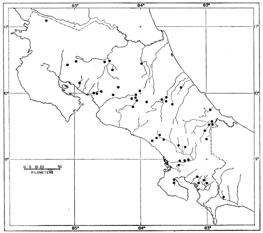
Fig. 5: Diagram showing the major associations of understory and overstory
vegetation in a trapping grid located south of Far View Ruins, Mesa Verde
National Park, Colorado.
[448]
As the forest floor begins to slope into the drainage, the ground becomes
rocky and shrubs assume more importance in the understory. Most of this
shrubby zone is on the slope; on the western side this zone abuts pinyon-juniper
woodland, and on the eastern side is bordered by Artemisia tridentata
in the sandy bottom of the drainage. Shrubs become more abundant and
pinyon and juniper trees become less abundant as one approaches the drainage.
In the vegetation maps, this brushy zone is delimited on the east by a heavy
line passing vertically through the middle of the grid (Figs. 5-8). The codominant
shrubs in the understory of this zone are Amelanchier utahensis,
Artemisia nova and Purshia tridentata. The three most abundant plants on the
ground are Artemisia ludoviciana, Chrysothamnus depressus and Penstemon
linarioides.
The drainage occupies most of unit N and parts of Units I, J and M.
Unit N is at the head of the drainage; the ground slopes rapidly southward
and the bottom of the drainage in unit J is approximately 50 feet lower than
in unit N. The canopy cover of the drainage is Artemisia tridentata (Fig. 5).
The same three plants that are most abundant in the ground cover of the slope
are also most abundant in the drainage.
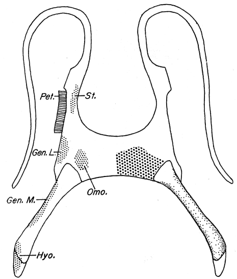
Fig. 6: Diagram showing the most abundant species of plants in the ground
cover of the trapping grid south of Far View Ruins.
[449]
The eastern slope of the drainage is covered with oak chaparral (Quercus
gambelii); this zone occupies parts of units J, L, M, and P. Artemisia ludoviciana,
Solidago petradoria, and Viguiera multiflora (goldeneye), are the
most abundant plants of the ground cover.
Mixed shrubs (Amelanchier, Cercocarpos, and Fendlera) form large
islands in the oak chaparral, in units K, L and P. The brushy areas of oak
and mixed shrub give way at the top of the slope to pinyon-juniper forest
with an understory of Artemisia nova and Purshia tridentata. The three
most abundant plants in the ground cover of the shrub zones are Solidago
petradoria, Balsamorrhiza sagittata, and Comandra umbellata. The eastern
part of unit O has Amelanchier utahensis in the understory, in addition to
Artemisia nova and Purshia tridentata (Fig. 5). The northeastern corner
of unit O is in pinyon-juniper woodland with an understory of Cercocarpos
montanus.
Fig. 7: Diagram showing the second most abundant species of plants in the
ground cover of the trapping grid south of Far View Ruins.
There are two relatively pure stands of sagebrush in the grid: one is in
unit N, and the other in unit F and part of unit G. As figures 5 to 8 show,
unit N has a relatively pure stand of Artemisia tridentata (big sagebrush),
[450]
with Artemisia ludoviciana, Agropyron smithii (western wheatgrass), and
Koeleria cristata (Junegrass), being most abundant in the ground cover.
Artemisia tridentata and Artemisia nova form the overstory in unit F and
part of G. The three most abundant plants in the ground cover there are
Chrysothamnus depressus, Solidago petradoria, and Penstemon linarioides
(Figs. 6-8).
Fig. 8: Diagram showing the third most abundant species of plants in the
ground cover of the trapping grid south of Far View Ruins.
Microclimates of Different Habitats
Four microclimatic stations were established in units D, F, L and M of
the trapping grid to record air temperatures and relative humidities at ground
level. These sites were chosen as being representative of larger topographic
or vegetational areas within the grid. Belfort hygrothermographs were installed
on June 10, 1964, and were serviced once each week through October
31, 1964, at which time the stations were dismantled. Each station consisted
of a shelter 18 by 9 by 11.5 inches, having a false top to minimize
heating (Fig. 9). The shelters were painted white. Several rows of holes,
each one inch in diameter, were drilled in all four sides of each shelter,
to provide circulation of air. The holes were covered by brass window
screening to prevent entry of insects and rodents. Preliminary tests with
several U. S. Weather Bureau maximum and minimum thermometers, suspended
one above the other, from the top to the bottom of the shelter,
revealed that there was no stratification of air within the shelters. Nevertheless,
each shelter was placed so that the sun did not strike the sensing
elements of the hygrothermograph inside it.
[451]
Fig. 9: (above) Photograph of microclimatic shelter built to house
hygrothermograph. False top minimizes heating, and ventilation holes
are covered with screening. (below) Photograph showing shelter in use.
[452]
Accuracy of the hair elements was checked by means of a Bendix-Friez
battery driven psychrometer, in periods when humidity conditions were
stable (on clear days the relative humidity is at its lowest limits and is
"stable" for several hours during early afternoon).
The four microclimatic stations were in the following places: 1) a stand
of big sagebrush near Far View Ruins; 2) a pinyon-juniper-muttongrass association;
3) a stand of big sagebrush at the head of a drainage; and 4) a
stand of Gambel oak on a southwest-facing slope of the drainage. Table 4
shows monthly averages of maximum and minimum air temperatures and
relative humidities at each of the four sites. Vegetation and microclimates
of the sites are discussed below.
Far View Sagebrush Site, 7,650 feet elevation
The shelter housing the hygrothermograph was next to the stake of station
F4a in the trapping grid (Fig. 10), in a stand of big sagebrush on the flat,
middle part of the mesa top, approximately 100 yards southwest of Far View
Ruins. The sagebrush extends approximately 200 feet in all directions from
the station (Fig. 5). Pinyon pine and Utah juniper trees are encroaching upon
this area, and scattered trees are present throughout the sagebrush. This area
is one of the habitats of P. maniculatus.
Sagebrush tends to provide less shade for the ground than pinyon-juniper
woodland, and therefore the surface temperatures of the soil rise rapidly to
their daily maximum. In mid-June, air temperatures rise rapidly from 6 A. M.
until they reach the daily maximum between 2 and 4 P. M. Shortly after
4 P. M. the air temperatures decrease rapidly and reach the daily low by about
5 A. M.
Relative humidities follow an inverse relationship to air temperatures; when
air temperatures are highest, relative humidities approach their lowest values.
Thus, on clear days, humidities decrease during the day, reaching a minimum
slightly later than air temperatures attain their maximum. Unless it rains,
the highest humidities of the day occur between midnight and 6 A. M.
Drainage Site, 7,625 feet elevation
This site was in the bottom of the drainage that runs through the eastern
side of the trapping grid, and through parts of units M, N, I, and J. The site
was at station M4d on a level bench at the head of the drainage (Fig. 11).
Southward from the station the drainage deepens rapidly, and the bottom
loses approximately 25 feet in elevation for every 200 feet of linear distance.
P. maniculatus lives here.
The microclimate of the drainage differs markedly from that of other
stations. The major difference is attributable to the topography of the drainage
itself. Nocturnal cold air flows from the surrounding mesa top to lower
elevations. A lake of cold air forms in the bottom of the drainage; the depth
of the lake depends in part upon the depth of the drainage. The same phenomenon
occurs in canyons and causes cooler night time temperatures on the
floor of canyons than on adjacent mesa tops (Erdman, Douglas, and Marr, in
press). Drainage of cold air into lower elevations affects both nocturnal air
temperatures and relative humidities. Table 4 shows that maximum air temperatures
in the drainage did not differ appreciably from those at other stations.
Mean minimum temperatures, however, were considerably lower in the drainage
than at the other sites. This phenomenon is reflected also in the mean air
temperatures at this station.
[453]
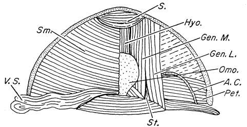
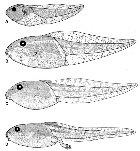
Fig. 10: (above) Photograph of microclimatic station at the Far View
Sagebrush Site, at trapping station F4a in the grid south of Far View
Ruins. Dominant vegetation is Artemisia tridentata.
Fig. 11: (below) Photograph of microclimatic station at the Drainage
Site, in the bottom of a shallow drainage at trapping station M4d of the
grid south of Far View Ruins.
[454]
The drainage site had the highest humidities of all stations each month in
which data were collected (Table 4). Relative humidities of 90 to 100 per
cent were common in the drainage, but occurred at other stations only in
rainy periods. For example, in the month of August, 26 of the daily maximum
readings were between 95 and 100 per cent at the drainage site, but at the
other stations relative humidities were above 95 per cent for an average of only
nine nights. Minimum humidities were about the same for all stations, since
they are affected by insolation received during the day, and not by the
drainage of cold air at night.
Oak Brush Site, 7,640 feet elevation
The station was in an oak thicket at trapping station L4a, 250 feet south and
50 feet east of the drainage site on a southwest-facing slope of about 30 degrees
(Fig. 12). The station was on the lower third of the slope, approximately 15
feet higher than M4d, the station in the bottom of the drainage. P. truei and
P. maniculatus occur together in this area.
Air temperatures and relative humidities at this station did not differ appreciably
from mean temperatures and humidities at the other stations. The
unusual feature is the lack of evidence of cold air drainage. The lake of cold
air in the bottom of the drainage apparently is too shallow to reach this station.
This site is near the head of the drainage, and the cold, nocturnal air probably
moves rapidly down slope into the deeper parts of the canyon, rather than
piling up at the shallow head of the drainage.
In spite of the shade afforded the ground by the oak brush, temperatures
reached the same maximum values as at the drainage site, owing to the orientation
of the slope. South-facing slopes receive more direct insolation throughout
the day and throughout the year than north-facing slopes and mesa tops
(Geiger, 1965:374). In Mesa Verde, south-facing slopes tend to be more
arid; snow melts rapidly, and most of this moisture evaporates. As a consequence,
south-facing slopes have less soil moisture and more widely-distributed
vegetation than north-facing slopes where snows often persist all winter and
melt in spring. (For a detailed discussion of climates on northeast-versus-southwest-facing
slopes in Mesa Verde, see Erdman, Douglas, and Marr, in
press.)
Pinyon-Juniper-Muttongrass Site, 7,600 feet elevation
The station was in the trapping grid at D5b (Fig. 13). The pinyon-juniper
woodland surrounding this site resembles much of the woodland on the middle
part of the mesa. The forest floor is well shaded by the coniferous canopy, and
muttongrass is the dominant plant in the ground cover. P. truei lives in this
habitat.
The climate at this site is moderate. Shade from the canopy greatly moderates
the maximum air temperatures during the day; minimum air temperatures,
however, are about the same as at the other stations (Table 4). Mean
temperatures are somewhat lower at this site than at the others because of the
lower maximum temperatures. Relative humidities do not differ markedly
from those at other stations.
Figure 14 shows hygrothermograph traces at all stations for a typical week.
An interesting phenomenon is illustrated by several of these traces. By about
midnight, air temperatures have cooled to within a few degrees of their nightly
low. At this time, heat is given up by the surface of the ground in sufficient
quantities to elevate the air temperature at ground level. This release of reradiated
energy lasts from one to several hours, then air temperatures drop
to the nightly low just before sunrise. A depression in the percentage of relative
humidity accompanies this surge of warmer air. On some nights winds
apparently disturb, or mix, the layers of air at ground level. On such nights
the reradiation of energy is not apparent in the traces of the thermographs.
Reradiation of energy is restricted to ground level, and traces of hygrothermographs
in standard Weather Bureau shelters, approximately four feet above
the ground surface, at other sites on the mesa top did not record it.
[455]
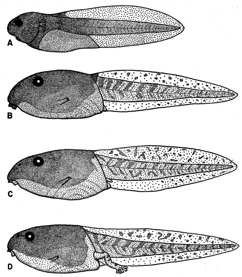
Fig. 12: (left) Photograph of microclimatic station at the Oak Brush Site, at trapping station L4a of the grid south of Far
View Ruins. (right) General view of the stand of Gambel oak in unit L of the trapping grid.
[456]
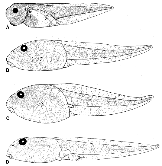
Fig. 13: Photograph of microclimatic station at the Pinyon-Juniper-Muttongrass
Site, at trapping station D5b of the grid south of Far View Ruins.
Grass in the foreground is muttongrass, Poa fendleriana.
The instruments used in this study were unmodified Belfort hygrothermographs
containing as sensing units a hair element for relative humidity and a
Bourdon tube for air temperatures. The hair element, especially, does not
register changes in humidity at precisely ground level; rather, it reflects
changes in the layer of air from about ground level to about a foot above.
Thus data from these instruments give only approximations of the conditions
under which mice live while they are on the ground.
Climatic conditions greatly influence trapping success. Larger numbers of
mice generally were caught on nights when humidities were higher than
average. Rain in part of the evening almost invariably resulted in more mice
of each species being caught. This was probably due to increased metabolism,
by the mice, to keep warm. Apparently the mice began foraging as soon as
the rains subsided; mice were always dry when caught after a rain. Few
mice were caught if rains continued throughout the night and into the daylight
hours.
[457]
Table 4—Monthly Averages of Daily Means for
Maximum, Minimum, and Mean Air Temperatures and Relative Humidities at Four
Sites in Mesa Verde National Park, Colorado.
| Site | Maximum Temps. | Maximum R. H. | ||||||||
| J | J | A | S | O | J | J | A | S | O | |
| Far View Sagebrush | 89 | 91 | 86 | 77 | 74 | 68 | 84 | 82 | 88 | 71 |
| Drainage | 86 | 91 | 85 | 78 | 78 | 87 | 94 | 93 | 96 | 84 |
| Oak Brush | 86 | 88 | 82 | 76 | 81 | 57 | 78 | 80 | 80 | 66 |
| Pinyon-Juniper-Poa | 75 | 80 | 74 | 66 | 64 | 59 | 83 | 82 | 88 | 58 |
| Minimum Temps. | Minimum R. H. | |||||||||
| J | J | A | S | O | J | J | A | S | O | |
| Far View Sagebrush | 42 | 53 | 50 | 42 | 31 | 18 | 24 | 25 | 29 | 21 |
| Drainage | 36 | 48 | 45 | 38 | 26 | 21 | 26 | 27 | 29 | 30 |
| Oak Brush | 42 | 52 | 50 | 42 | 32 | 19 | 25 | 30 | 31 | 21 |
| Pinyon-Juniper-Poa | 44 | 54 | 50 | 42 | 34 | 22 | 30 | 29 | 32 | 25 |
| Mean Temps. | Mean R. H. | |||||||||
| J | J | A | S | O | J | J | A | S | O | |
| Far View Sagebrush | 66 | 72 | 68 | 60 | 52 | 43 | 54 | 54 | 48 | 46 |
| Drainage | 61 | 70 | 65 | 58 | 52 | 54 | 60 | 60 | 62 | 52 |
| Oak Brush | 64 | 70 | 66 | 59 | 56 | 38 | 51 | 55 | 56 | 44 |
| Pinyon-Juniper-Poa | 60 | 67 | 62 | 54 | 49 | 41 | 56 | 55 | 60 | 42 |
[458]
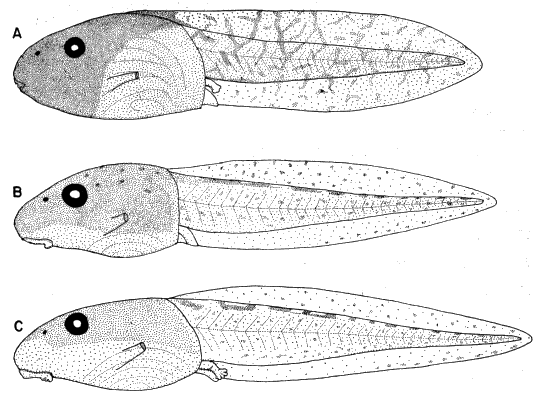
Fig. 14: Diagram of hygrothermograph traces showing daily progressions of
air temperatures and relative humidities at each of four microclimatic stations,
from the morning of July 1 through the morning of July 8, 1964. Slanting
vertical lines on each chart designate midnight (2400 Hrs.) of each day.
[459]
Nights of high trapping success usually were associated with days having
solar insolation below the average. Insolation was measured with a recording
pyrheliometer at a regional weather station (M-2) on the middle of Chapin
Mesa, at an elevation of 7,150 feet (Erdman, Douglas, and Marr, in press).
This station was approximately one mile south of the trapping grid; isolation
at this site would have been essentially the same as that received by the
trapping grid. Below-average isolation for one day indicates cloudy conditions,
which are accompanied by increased humidity, but may or may not be
accompanied by precipitation. Trapping on nights preceded and followed by
days of average or above average isolation with average humidities—indicative
of clear days and clear moonlit nights—did not yield appreciably higher
catches of mice than other nights. Hence there was no evidence that mice
tended to avoid, or to seek out, traps on clear moonlit nights.
On cold, humid nights in autumn numerous mice caught in Sherman live
traps succumbed from exposure, even though nesting material (kapok or
cotton) and food were in the traps. Occasionally mice succumbed to heat
when traps were inadvertently exposed to too much sunlight. Apparently
little heat is required to kill individuals of either species. Traps in which
animals died due to excessive heat usually were not hot to the touch; in most
instances the traps were checked before 9:00 A. M., several hours before the
sun caused maximum heating. Such individuals may have licked the fur of
their chests in an attempt to lower their body temperatures. Although mice
characteristically salivate before succumbing from heat, these individuals had
moist fur over the entire chest and upper parts of the front legs, indicating
licking. Mice killed by exposure to heat or cold usually were juveniles or
young; subadult and adult individuals of both species were more tolerant.
Older animals would be expected to have better homeostatic controls than
younger individuals.
Habitat Preference
In Mesa Verde P. truei and P. maniculatus occur together only at the
fringes of the pinyon-juniper woodland, where ecotonal areas provide less
than optimum habitats for both species. Almost all individuals of P. truei
occur only in pinyon-juniper woodland, whereas P. maniculatus occurs only
in more open habitats, such as grassy meadows and stands of sagebrush.
Pinyon mice were abundant in a variety of associations within the pinyon-juniper
woodland. The highest population densities were in pinyon-juniper
woodland having an understory of mixed shrubs. In such an association, Poa
fendleriana usually is the dominant grass in the ground cover. P. truei was
especially abundant along brushy slopes where mixed shrubs (Amelanchier,
Cercocarpos and Fendlera) were codominant with pinyon pines and Utah
junipers. The pinyon-juniper-mixed shrub area west of Far View Ruins was
almost optimum habitat for P. truei.
P. truei was abundant on the rocky ridge of Wetherill Mesa near Mug
House; the pinyon-juniper woodland here has a Cercocarpos understory, and
appears to provide close to optimum conditions for this species.
Not all associations of the pinyon-juniper woodland support large numbers
of P. truei. Pinyon-juniper woodland having a ground cover of Poa fendleriana,
and no shrubs, supports few mice; the woodland on Wetherill Mesa near Long
House is an example. Juniper-pinyon woodland having a Purshia tridentata
understory also supports only a few mice. Such areas occur on the southern
[460]
ends of the mesas and are characterized by widely-spaced trees and little
ground cover—a reflection of the relatively low amounts of precipitation received
by the southern end of the park.
P. truei was not found in grasslands on Navajo Hill, or in meadows at the
southern end of Moccasin Mesa. The old burned areas on the northern end
of Wetherill Mesa and on Morfield Ridge now support numerous grasses and
shrubs, but P. truei appears not to live there.
P. truei tends to avoid stands of sagebrush, or grasslands, lacking pinyon or
juniper trees. P. truei may venture into such areas while feeding. This species
is found in thickets of Gambel oak and in areas with an overstory of mixed
shrubs only when a living pinyon-juniper canopy is present, or when a woodland
adjoins these areas.
Rocky terrain apparently is not a requirement for P. truei, since much of
the pinyon-juniper woodland that is free of rocks supports large numbers.
Optimum habitat, however, had a rocky floor. In such places, rocks probably
are of secondary importance, whereas the shrubs and other plants growing on
rocky soils are important for food and cover. Rocks likely provide additional
nesting sites, and allow a larger population to live in an area than might
otherwise be possible.
In Mesa Verde the deer mouse, P. maniculatus, prefers open areas having
dense stands of grasses, or brushy areas adjoining open terrain. This species
lives in stands of big sagebrush; in grassy areas having an oak-chaparral or
mixed-shrub-overstory; and in grasslands without shrubs, such as on the southern
end of Moccasin Mesa. Pure stands of sagebrush did not support large
numbers of mice unless there was additional cover nearby in the form of
shrubs or oak brush.
Optimum habitats for P. maniculatus were on Navajo Hill, in the burned
areas on Morfield Ridge, on the northern end of Wetherill Mesa, and in the
grassy areas near the entrance of the park. The trapping areas in the first three
mentioned had heavy growths of grass and an overstory of shrubs.
Some individuals of P. maniculatus ventured into pinyon-juniper woodland
and entered traps. Such animals usually were found in places having a heavy
understory of sagebrush, or in disturbed places within the woodland.
P. maniculatus, but not P. truei, was taken in the arid pinyon-juniper-bitterbrush
stand on the southern end of Wetherill Mesa. P. maniculatus also
was present, in about equal numbers with P. truei, in a pinyon-juniper-muttongrass
stand north of Long House. Both of these localities supported
only a few mice.
P. maniculatus is found more frequently in pinyon-juniper woodland when
the population density is high, and when such woodlands adjoin grasslands or
sagebrush areas. As mentioned earlier, P. truei and P. maniculatus occur together
in ecotonal areas between the forest and grassy or brushy areas. In
Mesa Verde the deer mouse inhabits exposed grassy areas that have mostly
shrubs in the open canopy.
P. maniculatus is the first to colonize areas that have been burned; this
species invades such areas as soon as primary successional vegetation becomes
established. It can be stated that in general, P. maniculatus will be found in
the harsher, more arid habitats. If the habitat is so inhospitable that only a
few mice can survive there, P. maniculatus will be present. P. truei apparently
requires the more moderate conditions found in the pinyon-juniper forest, and
this species does not venture far from the edge of the forest.
[461]
Nesting and Nest Construction
Ten individuals of P. truei and three of P. maniculatus were followed to
their nesting places. Photographs were taken of the nesting sites before and
after uncovering. Plants or other materials used in their construction and any
commensal arthropods present were saved and later identified.
Nests of P. truei usually were associated with juniper trees. Dead branches
and trunks of juniper trees decay from the inside, and the resulting hollows
are favored sites for the nests. Pinyon pine trees tend to decay from the outside
and were not used as nesting sites by P. truei. Nests of P. truei were found
in hollow trunks and branches of otherwise healthy juniper trees, and in hollow
logs lying on the ground. The heartwood apparently rots rapidly in juniper
trees, but the sapwood remains intact for many years—even after the tree is
lying on the ground. For example, a part of the pinyon-juniper woodland on
the southern end of Chapin Mesa was burned in 1858, and the hollow trunks
of junipers were still standing in 1966. Almost all of the pinyon pine trees
that were killed by that fire have since decayed; their former presence is
verified only by the crumbling remnants of their trunks that lie on the ground
throughout the burned area.
The following accounts illustrate the preferences of the two species of mice
in selection of nesting sites:
No. 105, P. truei, adult. On July 22, 1964, after being released from a trap,
this female ran to a serviceberry bush 10 feet south of station I4d, preened
herself, ate a berry from the bush, and disappeared under a large rock at the
base of the bush. Subsequent excavation revealed a large nest composed of
grasses (Poa fendleriana, Sitanion hystrix, Agropyron smithii, Koeleria cristata),
and a few leaves of serviceberry. There were three entrances to the nest, one
on each side of the rock.
This mouse was captured again on August 12, 1964, released and followed
to a hollow juniper log 15 feet south of station C7b, and 245 feet from the
above nest. This log was dismantled, but no nest was found. A large number
of chewed juniper seeds around the log indicated that this mouse, or others,
had frequented the area.
On August 20, 1964, this female was followed to a large juniper log 20
feet northeast of station I4b. A small nest of shredded juniper bark was
found inside the log, and there were numerous nuts of pinyon pine and seeds
of Utah juniper that had been gnawed open. This site was about 320 feet from
that at C7b, and about 240 feet from station I4d (Fig. 15).
No. 118, P. truei, young. On August 29, 1963, this male ran into a hollow
branch of a partly dead juniper tree 15 feet south of station C5d. Part of
this branch had been sawed off at some earlier time, and a hole about one-and-a-half
inches in diameter was present in the center of the remaining part.
The branch was not dissected, but probing revealed that the hole extended far
into the branch and enlarged as it approached the trunk.
No. 177, P. truei, adult. This lactating female ran into the hollow trunk of
a juniper 10 feet north of station G7a. Both lateral branches of the main trunk
were rotten and hollow, but the tree appeared to be healthy. Chewed juniper
seeds were present in the trunks and around the base of the tree.
This female later ran to a juniper log 30 feet north of station N4d. Apparently
there was no permanent nest at this site (Fig. 15).
No. 178, P. truei, adult. This female ran into a hollow juniper tree 10 feet
south of station H3c. Hundreds of old juniper seeds, with their embryos
chewed out, were present at the base of the tree. The tree was not cut down.
No. 238, P. truei, adult. This male ran into a dead juniper log 10 feet south
of station O4b. Chewed juniper seeds were present on the ground, but no
nest was found in the log.
[462]
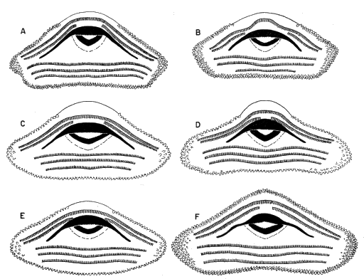
Fig. 15: Diagrams showing estimated home ranges of six individuals of two
species of Peromyscus, and location of these ranges in the trapping grid. Nesting
or hiding places are described in the text, and are indicated on each
diagram by an X. Shaded areas represent home ranges estimated from trapping
records for 1963; outlined, unshaded areas represent estimated home
ranges for 1964.
No. 241, P. truei, adult. This male ran into a small hole at the base of a
juniper tree 25 feet south of station G7c. The hole was at the fork of the
tree, four inches above the ground, and led to a large subterranean chamber in
the basal part of the trunk.
This male later ran into a dead juniper log lying on the ground 20 feet
southwest of station N3b. No nest was found in the log.
After another capture, this mouse ran to a small juniper log 40 feet southeast
of station G3d. There was a nest of shredded juniper bark and many
juniper seeds inside the log (Figs. 15-17).
No. 245, P. truei, adult. This female ran into a large, hollow juniper log
20 feet northwest of station D4d. No nest was seen, but chewed juniper seeds
were noted in and around the log (Fig. 15).
No. 251, P. truei, juvenile. This female ran into a dead juniper log beside
station P4b. Chewed cones of pinyon pine and chewed juniper seeds were on
the ground. A small nest of shredded juniper bark, and a few leaves of
serviceberry, were found inside the log. Chewed pinyon nuts and juniper seeds
also were present in the nest.
[463]
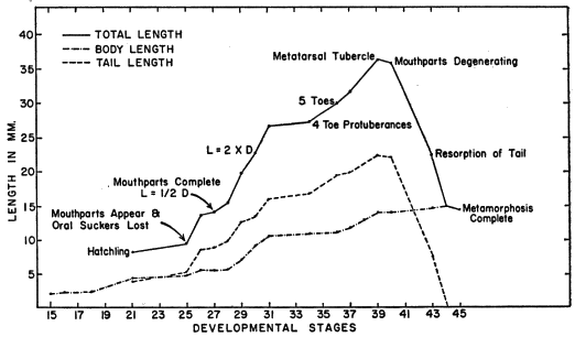
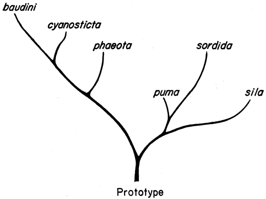
Fig. 16: (above) Photograph of juniper log at station G3d, which contained
the nest of P. truei # 241.
Fig. 17: (below) Photograph of dissected juniper log at station G3d,
showing the nest of P. truei # 241, at end of mattock handle. The nest of
shredded juniper bark contained chewed seeds of juniper trees.
[464]
No. 267, P. truei, juvenile. This male ran into a fallen juniper log 40 feet
southwest of station P7a and then disappeared into a hole leading under an
adjacent rock. Dissection of the log revealed many chewed juniper seeds inside
and beneath the log, but no nest. I did not overturn the large rock or
excavate under it.
No. 268, P. truei, adult. This pregnant and lactating female ran into a
hollow branch of a partly-dead juniper tree 10 feet south of station O7d. The
limb and base of the tree were hollow, and there were large numbers of
chewed juniper seeds nearby. Because of time limitations, the branch was not
dissected.
No. 74, P. maniculatus, juvenile. This female ran into a small circular hole
in the ground 13 feet north of station J3a. Excavation revealed that this
hole led into the abandoned tunnel of a pocket gopher (Thomomys bottae).
The tunnel was followed for about four feet, but no nest was found and the
tunnel led under a thicket of oak brush which made further excavation impractical
(Fig. 15).
No. 247, P. maniculatus, adult. This male was followed to a large nest
situated at the base of a stump and under a juniper log lying beside the
stump, five feet from station I2c. This large nest was built on the ground
and was constructed of grasses (Poa fendleriana, Stipa comata, and Koeleria
cristata), and contained a few leaves of Gambel oak. It was the largest nest
found. Chewed pinyon nuts were in the nest. (Fig. 15).
No. 276, P. maniculatus, juvenile. This male ran into a small hole at the
base of a dead juniper tree 40 feet north of station O2c. It would have been
necessary to cut the tree down to uncover the nest, and this was not deemed
to be worthwhile.
The preceding accounts indicate that, in Mesa Verde, nests of P. truei
usually are associated with hollow juniper logs or branches. In one instance
a nest of P. truei was found on the ground, under a rock. Shredded juniper
bark, and, in one case, grasses were the materials most commonly used for nest
building.
Individuals of P. maniculatus did not build nests in trees. One nest was
found under a stump and adjacent log. Another site was in the abandoned
tunnel of a pocket gopher, and a third was under a large rock. The only nest
that was unquestionably built by a P. maniculatus was constructed of grasses
and a few leaves.
It seems unlikely that competition for nesting sites between the two species
of Peromyscus affects the local distribution of each species. The analysis of
nesting sites suggests that P. truei is restricted, in Mesa Verde, by the
availability of fallen logs, hollow branches, or hollow trunks of juniper trees.
My observations lead me to think that within the pinyon-juniper woodland
there is a surplus of nesting sites for individuals of P. truei. Many juniper
trees have dead branches, and hollow juniper logs are abundant throughout
the forest. It is inconceivable to me that the population of P. truei could
reach densities sufficient to saturate every nesting site available to them in
the trapping grid.
Sagebrush areas, or brushy zones adjacent to the pinyon-juniper woodland
usually do not contain juniper logs; when hollow juniper trees or logs are
not available, P. truei is not found as resident of such areas. As mentioned
earlier, individuals of P. truei may venture into such areas to feed if they
are adjacent to pinyon-juniper woodland.
An individual of P. truei may have more than one nest within its home
range (for example Nos. 105 and 241 cited above). Each mouse probably
has refuges, each containing a nest, strategically located in its home range.
Thus, if a mouse is chased by a predator, or by another mouse, it need not
[465]
return to its main nest, but can seek refuge in one of its secondary nests.
These secondary nests were small and were invariably constructed from
shredded juniper bark. Some of these nests were little more than a scant
handful of shredded bark that formed a platform to sit upon. Other nests
were larger and ball-shaped, with one opening on the side. All of the
secondary nests that were found were inside hollow juniper logs. The
bark used in construction of the nests had, in each case, been transported
from nearby living trees. The logs had previously lost their bark through
decay.
The evidence indicates that these secondary refuges are prepared with
considerable care. Not only is the bark transported for some distance, but
it is shredded into a soft mass of fibers. When a mouse first establishes
itself in a new area, perhaps it begins several such nests before settling upon
the most favorable site. The less desirable sites, if still within the animal's
range, are then available (barring competition by a new inhabitant) for
outlying refuges.
My data do not indicate whether individuals of P. maniculatus use a similar
arrangement of nests within their home ranges. The population of P.
maniculatus was sparse in the trapping grid, and the habitat these mice occupied
was such as to make following them extremely difficult.
In captivity, both species constructed nests that were indistinguishable
to me, when the mice were given cotton, kapok, or pieces of burlap as
building material. The cotton or kapok was used directly, but the burlap
was shredded into a fine mass of fluffy fibers. The burlap seemed to me
to be the best building material, for it maintained its shape best.
Both species constructed nests that resembled inverted bowls. Solitary
mice naturally built smaller nests than those built by females with young.
The entrance to the closed nests varied; often the female would bolt
through the side of the nest where there was no opening. Sometimes the
mice would exit and enter through the top of the nest. In some cases it
appeared that the entire nest was closed; probably the occupant had closed
the entrance. Such a closed nest would have the advantage of greatly moderating
the microenvironment within the nest, and would allow the animal
within to remain comfortable with a minimum expenditure of energy. The
larger nests found in the trapping grid resembled those built by captives.
Nests built of grasses were always larger than those built of juniper bark.
Juniper bark is as easily worked into nests as are grasses, in my judgment.
Therefore, difficulty of construction of nests from this material probably does
not account for the smaller size of the nests composed of bark. I think the
difference in insulating characteristics between the two materials probably
accounts for the difference in size of the nests.
Reproduction
In Mesa Verde, Peromyscus reproduces from April through September.
Reproduction is greatly reduced in the autumn, and most females complete
reproduction before October.
Ten of the 20 females of P. maniculatus, taken in May, contained embryos;
five others were lactating. Lactating and pregnant females were collected on
May 5, 1962, indicating that reproduction in some females began in early
April. In September, 15 of 34 females were pregnant or lactating, whereas in
October only two out of 15 females of P. maniculatus were reproducing. Only
[466]
one female of P. maniculatus was found to contain embryos in October. This
large adult was taken on October 3, 1963, and had six embryos, each five
millimeters long. She probably would have produced a litter later in October,
and would have been nursing into November. A report of October breeding
in north-central Colorado described nine of 23 females of P. maniculatus as
being in a reproductive state; seven were lactating and one was pregnant
between October 26 and 31, 1952 (Beidleman, 1954:118).
In the Museum of Natural History, the University of Kansas, there are 35
females of P. maniculatus more than 144 millimeters in total length taken
from Mesa Verde in November, 1957 (Anderson, 1961:53). None of these
contained embryos, and no pregnant females have been taken from the park
in November.
P. truei and P. maniculatus reproduce at about the same time. A female of
P. truei prepared as a specimen on May 10, 1964, contained four embryos,
each 20 millimeters long, indicating a breeding time in mid-April. Svihla
(1932:19) reported the gestation period for non-lactating P. truei to be 25 to
27 days and for lactating individuals, 40 days. Lactation tends to increase
the gestation period of other Peromyscus by about five days (Asdell, 1964:266).
The gestation period of nine non-lactating females of P. m. rufinus was reported
by Svihla to be 23 to 24 days. Lactation increased the length of the period of
gestation in this subspecies to between 23 and 32 days (mean for seven
females 26.57 ± 0.73, Svihla, 1932:19).
Females of P. truei were observed in various stages of reproduction from
June through September. Ten of the 20 females of P. truei taken in September
were reproducing; four contained embryos and the other six were lactating.
In October, only one of 17 females caught in snap traps was lactating. Lactating
females were caught in live-traps as late as October 23, although most
females had ceased reproduction by then. No pregnant or lactating females
were observed in November.
In P. maniculatus, puberty has been placed at 32 to 35 days for females
weighing 13 grams, and in males at from 40 to 45 days, at weights of 15 to 16
grams (Jameson, 1953:45). In P. truei, the weight of the testes is reported
to rise in March and diminish through September, with accessory organs
following the same cycle (Asdell, 1964:267). Young of P. truei nurse for
about one month, although some litters may not be weaned until 40 days of
age. Young of P. maniculatus are weaned between 22 and 37 days of age
(Svihla, 1932:30).
Twenty-six pregnant females of P. maniculatus, taken in the breeding
seasons of 1961-1964, contained from one to eight embryos each; the mean was
4.65 ± 1.67. Other investigators have found similar mean values in this species
(Asdell, 1964:266).
Thirteen females of P. truei taken in the breeding seasons of 1961-1964,
contained from three to six embryos each; the mean was 4.0 ± .912. Svihla
(1932:25) reported litter sizes, at birth, of two to five and a mean of 2.84,
in 19 litters. Other investigators have reported litter sizes of one to five with
a mean of 3.4, and one to six with a mean of 3.6 (Asdell, 1964:268). Apparently
P. truei does not have more than six young per litter.
In captivity, females of both species began reproduction in early February.
These captives had been kept for several months at a temperature of 21 degrees
Centigrade, and on a daily photoperiod of 15 hours. Some captive males had
enlarged, scrotal testes in January; the extended photoperiod and warm temperature
[467]
probably influenced the breeding condition. In both species testes
of wild males caught in autumn after late September and on through the winter
were abdominal, except for one male of P. maniculatus which had enlarged,
scrotal testes on October 15.
Dates at which different animals arrived at breeding condition varied, in
part owing to subadults (young of the year) appearing in the catch from
early summer to late autumn. Some adult females appeared to be pregnant
or lactating throughout much of the summer and early autumn, whereas other
females, that were caught a number of times, apparently reproduced only once
in the summer.
Some females may fail to breed even though they are mature enough to do
so. One female of P. truei captured eight times (August 30 to September
20) was a juvenile when first caught, and was classed as young (in postjuvenal
molt) on September 10. She did not reproduce in her first breeding season,
unless she did so after September 20, which is unlikely. Another female of
P. truei was an adult when first caught, and was caught 12 times (August 21
to October 25). At no time were her mammae enlarged and she was not
lactating or pregnant. It is improbable that she reproduced earlier in the
season, for teats of mice that have reproduced earlier usually are enlarged to
such a degree that previous parturition is clearly indicated. It was surprising
to catch a female, of any age, 12 times in two months without sign of reproductive
activity.
Only one female of P. maniculatus did not show reproductive activity. She
was a juvenile on July 19 when first caught; a subadult on August 28 when
caught the third time, and an adult on October 23 when caught the fifth time.
Burt reported a rest period of a month or more in the summer, in Michigan,
during which many females of P. leucopus did not reproduce. They began
to breed again in late summer at about the time when young of the year
began reproducing (Burt, 1940:17, 19). Abundant mast was correlated with
reproductivity in autumn, according to Jameson (1953:54), who thought that
"food is a basic determinant of the autumn reproduction" of P. leucopus.
Little has been written about the length of time males remain in breeding
condition. Difficulties in determining breeding condition are many. Fertility
customarily is determined by sectioning testes and noting the presence or
absence, and relative abundance, of sperm. This procedure necessarily sacrifices
the individual and indicates the breeding condition at only one moment
and for only the individuals sacrificed. My observations of males caught a
number of times in live traps shed some light on the breeding condition of
males, but the investigator is likely to err in extrapolating physiological data
from morphology when he notes whether the testes are abdominal or scrotal
and whether they are enlarged or small. It was assumed that testes that have
not descended, and that lie within the abdominal cavity, are not capable of
producing viable sperm. This is the condition in most juveniles, and in all
males during winter. As the breeding condition is attained, testes descend
into the scrotum. Soon the testes and their accessory organs enlarge and are
readily apparent.
Howard (1950:320) reported that numerous males of P. leucopus sired
litters when their testes appeared to be abdominal, and therefore questioned
whether the criterion of descended testes is valid as an indicator of breeding
condition. My captive males of P. maniculatus and P. truei did not sire litters
when their testes were abdominal, even though such males were left with
[468]
adult females for as long as four to five months (August through December).
Captive pairs of both species yielded no evidence of reproductive activity until
January when, as mentioned earlier, some of the males had scrotal testes.
Young were born first in early February, although their parents had been
confined together since the preceding August. Jameson reported the testes
of fecund males of P. maniculatus as almost always 8.0 millimeters or larger
(Jameson, 1953:50). Testes that are at least partly scrotal must be considered
as being capable of producing motile sperm, even though this may not be the
case for all individuals.
Toward the beginning and end of the breeding season the testes and accessory
organs of wild mice were small and probably produced few if any sperm.
At these times some males apparently were so frightened by being handled
that the testes were retracted into the inguinal canals. It would have been
easy to consider such males as having abdominal testes when in fact they
did not. In such cases the scrotum usually was noticeably enlarged; it was
found also that in many cases the testes returned to the scrotal position if
the mouse was held gently for a few minutes. Careful handling of animals
was found to prevent, or at least retard, retraction of the testes. Retraction
of the testes from the scrotum was not a problem at the height of the breeding
season when the testes were engorged.
I had originally assumed that all adult males would be fertile throughout
the breeding season, and that any males with abdominal testes would be
subadults or young of the year. This assumption was an oversimplification;
all adult males did not reach breeding condition at the same time of year.
My data do not support a firm conclusion, for it is difficult to follow non-captive
individuals throughout a breeding season, owing to sporadic appearance
of animals in traps. Nevertheless, observations of mice that were trapped
a number of times indicated the following:
1) Some adult males that had abdominal testes in the middle of July
reached breeding condition as late as late August and even late September.
2) Some juvenal males had scrotal testes at the time their postjuvenal molt
was just beginning to be apparent on their sides. Most juvenal males did not
have scrotal testes, and many juveniles that appeared repeatedly in traps
from mid-July through late October did not attain breeding condition. A
mouse that was a juvenile in mid-July must have been born in mid-June.
3) Apparently animals born early in the breeding season may reproduce
later in that season, whereas those born later in the breeding season tend
not to breed until the following year.
Possibly cooler evening temperatures in July and August, due to the
relatively larger amounts of precipitation in those months, inhibit reproductive
development of late-born young. Most plants have ceased vegetative growth
and have produced seeds by this time; but the interrelationships between
growing seasons, climatic conditions, and reproductive physiology are unknown.
Only one adult of each species had scrotal testes after late September;
the P. truei had scrotal testes on October 24, 1963, and the P. maniculatus
had scrotal testes on October 15 of that year.
[469]
Growth
Growth of captive P. maniculatus and P. truei is discussed in several reports.
One of the most complete is that of McCabe and Blanchard (1950)
on P. m. gambelii and P. t. gilberti in California. A detailed discussion of
the dentition in P. truei and wear of the teeth in different age groups is
given by Hoffmeister (1951). Molt in these species has been considered by
a number of authors (Collins, 1918; McCabe and Blanchard, 1950; Hoffmeister,
1951; Anderson, 1961). The report by McCabe and Blanchard is
valuable because molt is compared between the two species from the first
to the twenty-first week of postnatal development.
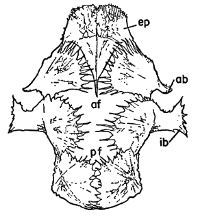
Fig. 18: Scatter diagram of postnatal growth of captive mice, showing increase
in length of bodies from birth to 70 days of age. The records for P.
truei represent 11 individuals of five litters; those for P. maniculatus represent
17 individuals of four litters.
[470]
The thoroughness of the above-mentioned studies is readily apparent to
those who have worked with mice of the genus Peromyscus. Nevertheless,
the ecology of local populations of P. maniculatus and P. truei as reported
for the San Francisco Bay area (McCabe and Blanchard, 1950) has little
relationship to the ecology of mice of other subspecies of these species, in
southwestern Colorado. Indeed, the preferred habitats, and to some extent
the behavior, differ strikingly in Colorado and California.
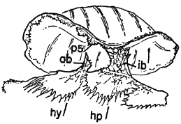
Fig. 19: Graphs showing postnatal growth of solitary captive individuals of
P. truei and P. maniculatus, representing the only young in each of two litters.
Figures 18 and 19 show that some litters grow appreciably faster than
[471]
others, but the end results are about the same. Since the young were measured
at irregular intervals, statistical procedures for calculating confidence
limits of the curves were not applicable.
Solitary young reared by one female of each species, attained maximum
size more rapidly than animals having litter mates (Fig. 19). Nevertheless,
solitary individuals and individuals from litters all reach essentially the same
size 50 days after birth.
The gestation time of P. truei is several days longer than that of P. maniculatus,
and the young of truei are fewer and heavier than those of maniculatus.
As would be expected, truei remains in the nest longer and nurses longer than
maniculatus.
Young of each species grow rapidly for the first month, and attain, in
that time, the largest percentage of their adult size; they grow rapidly up to
sometime between the thirtieth and fiftieth days. Thereafter the rate of
growth diminishes and the animals begin to gain weight rather than continuing
to extend the lengths of the body and appendages.
Figure 19 reveals that the appendages of young maniculatus attain most
of their length about a week earlier than those of truei. Young truei acquire
mobility and coordination somewhat later than young maniculatus, but both
species are seemingly equal in these respects by about the end of the second
week.
Length of gestation period, number and size of embryos, amount of time
spent in the nest, and time required for bodily growth are all of major
importance in determining the relative success of truei and maniculatus.
These parameters will be considered further in the discussion.
Parental Behavior
In the laboratory, pregnant females were supplied with either kapok, cotton,
or a piece of burlap with which to make a nest. The kapok or cotton was used
directly by the mice in constructing a hollow, compact, moundlike nest. When
burlap was used for nest building, the female first completely frayed the cloth
by chewing it into a fluffy mass of fibers.
When the top of a nest was opened to inspect young, the female would
attempt to pull the nesting material back into shape by means of forefeet and
teeth. The mother's defensive posture was to cover the young with her body,
often lying over them and facing upward, toward the investigator. In this semi-recumbent
position, the female would attack the investigator's fingers with her
forefeet and teeth. Often the female would stand bipedally and use the forefeet
and teeth to mount the attack. If at this time a young chanced to wander
away from the mother, she would quickly pick it up and place it in the nest
at her feet.
When disturbed, females of both species, but especially P. maniculatus,
often dove headlong under their nest or into the wood shavings on the floor
of the cage. This type of retreat was most often used when young were nursing.
Time is required even by the mother to disengage nursing young, and this
mode of escape is the most expedient. The mother disengaged nursing young
by licking around their faces and pushing with her paws.
Nursing females of both species tolerated the male parent in the nest. A
male and female often sat side by side in the nest and by means of their bodies
participated in covering the young. Males were not observed to attempt any
[472]
defense of the nest, or of the young. Females were tolerant of older young in
the nest when another litter was born and was being nursed. In one nest, a
female of P. truei gave birth to a litter of three when her older litter was 29
days old. The three older young continued to nurse until they were 37 days
old, at which time they were removed from the cage. The female appeared
tolerant of this nursing by members of the older litter, but appeared to give
preference to the wants of the younger offspring.
One female of P. truei lost or killed all but one young of her litter; at about
the same time, a P. maniculatus and all but one of her young inexplicably died.
Since the remaining young maniculatus, a male, was just weaned and was
considered expendable, I placed him in the cage with the female truei and her
33-day-old, male offspring. The reaction to the newcomer was unexpected.
The female immediately covered the P. maniculatus and her own young and
prepared to defend them against me. Later, when the P. maniculatus was
disturbed, he had only to emit a squeak and the female truei would run to
cover and protect him. When the young male of P. truei was 69 days old the
female kept him out of the nest, but still kept the male maniculatus in the
nest with her. Although the female was somewhat antagonistic to her own
young, she did not injure him, but only kept him out of the nest. The male
truei was left in the cage with his mother and the P. maniculatus from September
23 to December 10. None of the mice had any apparent cuts on the ears
or tail to indicate fighting. As much as seven months after the P. maniculatus
was introduced into the cage, the female truei continued to cover him with
her body whenever there was a disturbance. The male maniculatus not only
tolerated this attention, but ran under the female truei when frightened.
"Adoption" of young of another species has been reported for a number of
animals, but, without further evidence, it is not possible to postulate that such
adoptions occur between species of Peromyscus in nature.
Young males are tolerated by their mothers after weaning. One young male
maniculatus was left in the cage with his mother from the time of his birth
in autumn until late February of the following year. A litter was born on
February 24. A young male P. truei was also left in the cage with his mother
until he had acquired most of his postjuvenal pelage; the female and male
usually sat together in the cage.
Females of both species sometimes eat their young when the young die
shortly after birth. One female of each species killed three of her four young,
and ate their brains and viscera. In one of these cases, the female, of P.
maniculatus, also died; the female of P. truei was the same one that adopted
the surviving P. maniculatus. The female truei continued to nurse her one remaining
young for at least several days after killing three of his litter mates.
A reason for this cannibalism might have been that I had fed these mice for
several weeks on a mixture of grains low in protein content. Inadequacy of
this diet for nursing females may have caused them to become cannibalistic. The
feed of all captives was changed to Purina Laboratory Chow after the young
were killed.
Transportation of Young
Females of both species transported their young either by dragging them
collectively while the young were attached to mammae, or by carrying them
one at a time in the mouth. Since mice of the subgenus Peromyscus have three
[473]
pairs of nipples, they probably transport only six young collectively. Svihla
(1932:13) has stated that both pectoral and inguinal teats are used in transporting
young, in contrast to Seton's reputed assertion that only inguinal nipples
were used. But Svihla neglected to cite Seton's complete statement. Seton
(1920:137) recorded a litter of three as using only the inguinal mammae, but
on the following page recorded the use of both inguinal and pectoral mammae
by another litter of four. My findings agree with those of Svihla. Nursing
females of both species were removed periodically from cages by lifting them
by the tail. The young would hang onto the mammae and the female would
clutch the young to her with all four feet. Young two weeks old or older
crawled behind the mother while nursing.
The method of transporting young in the mouth has been mentioned by
Seton (1920:136) and described by Lang (1925) and Hall (1928:256). These
authors report that the mother picks the young up in her paws, and places it
ventral-side up in her mouth, with her incisors around it. The young are not
picked up by the skin on the nape of the neck, as are the juveniles of dogs
and cats. I have found that females of both species of Peromyscus carry their
young ventral-side up in their mouth while the young are small, and sometimes
when the young are older. Generally, when females of P. truei moved
young weighing more than 10 grams, the female grasped the young from the
dorsal side, across the thorax just posterior to the shoulders, and held them
with the incisors more or less around the animal. Perhaps this method was
used with older young because of the observed tendency of the larger young
to resist being turned over and grasped from the ventral side, and because
their increased weight would have made it difficult, if not impossible, for the
mother to pick them up with her paws. The young rarely resisted the efforts
of the mother to move them by this method; when grasped across the thorax
by the mother, the young would remain limp until released. Some females of
P. truei would drag almost fully grown young back into the nest in this
manner. I have not observed older young of a comparable age to be moved
by females of P. maniculatus. The females of P. maniculatus appear to be
somewhat less concerned than those of P. truei for the welfare of their young
once they are mobile and close to being weaned.
The following listing describes changes in postnatal development of young,
of each species, from birth to nine weeks of age.
| P. truei | P. maniculatus |
| FIRST WEEK: At birth, young are helpless, red overall, small with wrinkled skin. Pinna of ear folded over and closed; eyes closed; digits not separated from rest of foot. | At birth, young are helpless, red overall, smaller than P. truei, skin wrinkled. Ear, eyes, and digits as in P. truei. |
| Redness diminished by fourth day. | Redness decreases and disappears by fourth day. |
| Hair apparent by fifth day; dorsal one-half or two-thirds of body more darkly pigmented than venter by fourth day. | Hair apparent by fourth day; body bicolored by end of week. |
| Young squeak loudly and suck; sometimes crawl, but drag hind legs. | Young squeak loudly; sucking more pronounced than in P. truei; may crawl, but drag hind legs. |
| SECOND WEEK: Appreciable increase in size; head about 60 percent larger than at birth, by 14th day, and still large in proportion to body. | As in P. truei. [474] |
| Toes on hind foot separated more from foot. | As in P. truei, but somewhat more advanced. |
| Body well haired by end of week; dorsum dark gray, venter whitish; tail bicolored in most, but not haired. | Body well haired by end of week; dorsum dark gray with brownish tint; venter whitish; tail bicolored in most, but not haired. |
| Pinna of ear unfolded and open by end of week. | As in P. truei, but developmentsomewhat more advanced. |
| Through day 10, use hind legs to push, but by end of week use legs to crawl; difficult to hold, squirm but do not bite. | Crawl well by end of week; difficult to hold, squirm but do not bite; agile. |
| Walk behind mother while nursing; agile. | |
| THIRD WEEK: Eyes open on 16th to 21st day. | Eyes open on 16th to 20th day, partly open earlier. |
| Gray pelage of dorsum brownish. Apparently there is a molt line progressing posteriorly from nose; the molt line has moved to shoulder region by end of week; pelage anterior to line browner, grayer posterior to it. | Pelage of dorsum brownish; molt line across shoulders progressing posteriorly; browner anterior to line, grayer posterior to it. |
| Tail haired and weakly bicolored in some individuals by end of week. | Tail haired and bicolored in all individuals. |
| Young walk and jump well; squirm but rarely bite. | Young walk and jump well; fight and bite when handled. |
| FOURTH WEEK: Begin to eat solid foods at 23-29 days, but also nurse. | Some young eat grain by 24th day; others continue to nurse. |
| Molt line about 3/4 inch posterior to head. Juvenal pelage completed by end of week. Some young have brownish hair on front legs. | Juvenal pelage complete; no sign of postjuvenal molt. |
| Young roll over on backs and use feet to ward off litter mates that are dropped into nest, or into container, with them. | As in P. truei; also, all jump well, and fight fiercely when handled. |
| FIFTH WEEK: Young weaned on 30th to 40th day; some nurse beyond 30th day if female is lactating. | All young weaned before or by end of week; none observed to nurse beyond 30th day, even if female is lactating. |
| Juvenal pelage complete and no postjuvenal molt apparent on dorsum. | Juvenal pelage complete; postjuvenal pelage not apparent on most, but probably present on all, and concealed under juvenal pelage. |
| SIXTH WEEK: Postjuvenal pelage apparent in most individuals under juvenal pelage, especially along lateral line. | Postjuvenal molt apparent in most young; almost complete in some, except above tail and on flanks. [475] |
| SEVENTH WEEK: Postjuvenal pelage apparent in most young; in some the molt line has progressed well up on the sides, but not to mid-dorsum. | Postjuvenal pelage apparent in all young; less distinct molt line than in P. truei. |
| EIGHTH WEEK: All individuals growing; total lengths of 156-170 millimeters; weight 17-22 grams. | Growth completed in some individuals; those in larger litters have total lengths of 128-144 millimeters; weight 14-17 grams. |
| NINTH WEEK: Testes partly scrotal in one male on 59th day. | "Scrotum in season usually large, vaginae open, evidence of coitus common." (McCabe and Blanchard, 1950:39). |
| New brown pelage encroaching on saddle and on hind legs; postjuvenal molt completed in some individuals by eleventh week. | Postjuvenal molt completed in some individuals by end of week. New pelage tends to be concealed under juvenal pelage longer than in P. truei. |
Changes Owing to Increase in Age
Increase in length of limb bones, changes in proportion of bones in the skull,
eruption and degree of wear of teeth, and changes in pelage can be used to
ascertain relative age. Different investigators might choose different limits for
the three categories young, subadult, and adult. Museum specimens were
assigned to one of five age groups listed below mostly on the basis of tooth
wear, essentially as described by Hoffmeister (1951:1).
Juvenile: M3 just breaking through bony covering of jaw or showing no
wear whatsoever.Young: M3 worn smooth except for labial cusps, and M1 and M2 showing
little or no wear.Subadult: M3 worn smooth; labial cusp may persist, but is well worn; M1
and M2 having lingual cusps worn, but not smooth; labial cusps showing
little wear.Adult: Lingual cusps worn smooth and labial cusps showing considerable
wear; labial cusp of M3 may persist.Old: Cusps worn smooth; not more than one re-entrant angle per tooth
discernible, frequently none.
For live animals examined in the field, criteria based on pelage and breeding
condition were used, as follows:
Juvenile: Only gray, juvenal pelage present.
Young: Subadult pelage apparent on lateral line or on sides; body usually
smaller than in adults.Subadults: Subadult pelage having mostly replaced juvenal pelage; mice
often as large as adults; testes of males often abdominal in breeding
season; gray juvenal pelage may persist on head of some individuals.[476]
Adult: Adult pelage present; body usually largest of all animals in population;
females may have enlarged mammae from nursing previous litters;
testes of males usually scrotal in breeding season; gray pelage may be
present on head of some individuals.
Old individuals in the field could not be distinguished from adults; hence
any animals that appeared older, or more developed, than subadults were
classified as adults.
In P. truei, subadult pelage appears first on the lateral line or on the flanks;
new pelage is ochraceous and contrasts markedly with the gray juvenal coat.
In P. maniculatus, the subadult pelage contrasts less with the juvenal coat; the
new pelage progresses from anterior to posterior over the body in the same
manner as in truei, but replaces the juvenal coat in a less distinct manner than
in truei. As a result, contrast often is lacking between juvenal and subadult
pelages in maniculatus making it difficult to assign an individual to one of these
two age categories when examined in the field. In museum specimens, the
subadult pelage is much more noticeable because it can be compared with the
pelages of other specimens. The subadult pelage in P. maniculatus is duller
than the adult pelage: In P. truei the subadult and adult pelages appear to have
an equal sheen.
In early winter, the postjuvenal pelage acquired by young individuals of
P. truei was thick and luxuriant and indistinguishable from the winter pelage
of adults. My observations lead me to conclude that individuals born late
in the breeding season molt from juvenal summer pelage directly into winter
adult pelage. Technically, this new coat is the postjuvenal one, yet it cannot
be distinguished as such after the molt is completed.
Anomalies and Injuries
Anatomical anomalies were rare in the individuals of Peromyscus that I
examined. When anomalies were found they were striking, principally because
of their low rate of occurrence.
One female of P. truei, born in captivity, had a congenital defect of the
pinna of the right ear, noted on the fifteenth day after birth. Closer examination
then and later revealed that the pinna was normal in all respects except
that the tip was missing. The tip showed no evidence of injury. When the
mouse was subadult, this defective pinna was approximately half as long as
the normal pinna. The topmost part of the defective pinna was somewhat more
constricted in circumference than the normal one.
On September 11, 1963, a subadult male of P. truei was captured that had
five functional toes on its right front foot, the only one of more than 175
individuals caught and handled in the field that exhibited polydactyly. The
front foot was examined closely in the field, but it could not be determined
how or where the extra bones of the sixth toe articulated. Peromyscus normally
has four full-sized toes on each front foot, and a small inner toe hardly more
than an enlarged tubercle, having no nail.
A few mice of both species had broken toes or claws torn off. Such injuries
were more common on toes of the hind foot. In several instances the toes
were shortened, as if by marking, although the animals concerned had been
[477]
marked earlier by clipping toes other than the injured toes. The reason for
these injuries is not apparent, although they could have been caused by
fighting, or from having been caught in doors of Sherman live traps.
Toes of several mice were swollen and inflamed due to small glochids of
cacti that were stuck in them. Apparently the mice had stepped on the glochids
by chance, for I found no evidence that Peromyscus of either species
eats cacti.
One P. truei had a broken tail; three other individuals had tails about one-half
normal length. One P. maniculatus had a shortened tail. Some of these
injuries probably were caused by the Sherman live traps; several individuals
of P. truei were released after having been caught by the tail by the spring-loaded
door of these traps.
On October 17, 1963, an adult P. truei had a bleeding penis; when this
mouse was recaptured on October 25, the injury was healed.
Losses Attributed to Exposure in Traps
Observations of wild mice caught in live traps suggest that metabolic
maturity is reached later than physical and reproductive maturity. In such
trapping, it became apparent that juvenal and young mice suffered from
exposure to cold and to heat much more than did subadult or adult mice.
Although traps were carefully shaded and ample nesting material and food
provided, some mice died in the traps. An overwhelming majority of these
mice were juveniles and young.
Traps were checked in the morning, both in the summer and autumn, yet
mice died in traps that were barely warm to the touch, in summer, and cool
to the touch in autumn. Older mice frequently were found in traps that
were warm, or even hot, to the touch; yet the older mice rarely died in such
traps. Apparently the tolerance of adults is much greater to heating and
chilling. Greater bulk and perhaps longer pelage in adults might provide
sufficiently better insulation to account for this difference.
Occasionally juvenal mice were found in traps in a sluggish and weakened
condition, especially in autumn when nights were cool. In such cases the
mice were either cupped in the hands and warmed until lively enough to fend
for themselves, or, if especially weakened, were taken to the laboratory. None
of such animals that were returned to the laboratory lived for more than two
weeks. Most of those released in the field did not reappear in the traps.
I conclude that juvenal and young mice placed under stress by overheating
or cooling die immediately or live only a few days. Subadult and adult
animals tolerate more extreme conditions of overheating or cooling, presumably
because they are able to regulate their internal temperature better,
by either losing or retaining heat more effectively.
Mice found dead in overheated traps had salivated heavily, and may also
have licked the fur on their chests to increase heat dissipation. One such
adult, of P. truei, had a wet chest when he was taken from a warm trap;
when released, this mouse ran to a nearby plant of Comandra umbellata, and
ate a few of the succulent leaves before running off. This individual was
trapped several times later in the summer, and apparently suffered no ill
effects from the exposure.
[478]
Dental Anomalies
Abnormalities in the formation and occlusion, or decay of teeth, are relatively
rare in wild mammals. Of all bodily structures, the teeth apparently
are under the most rigid genetic controls; they form early in the embryo and
follow rigidly specified patterns in their ontogeny. Apparently any deviation
from the normal pattern of tooth formation is quickly selected against. All
specimens of P. m. rufinus and P. t. truei in the collection of the Museum of
Natural History at the University of Kansas, and in my collection, were
examined for dental anomalies. A total of 317 specimens of P. m. rufinus
and 54 specimens of P. t. truei were examined. The following specimens
were found to have abnormalities:
K. U. 69361, P. maniculatus, adult: Small bundles of plant fibers are
lodged between all upper teeth and have penetrated the maxilla anterior to
the left M1. The maxillary bone is eroded away from the roots of all teeth.
The anteriormost roots of both lower first molars are almost completely exposed,
because the dentary has been abraded away.
K. U. 76041, P. maniculatus, young: A piece of plant fiber is wedged
between the left M2 and M3. The maxillary bone has eroded away from
around the roots of M3, indicating the presence of an abscess in this area.
K. U. 69362, P. maniculatus, adult: All teeth in the lower right tooth-row
are greatly worn, especially on the lingual side. The labial half of the right
M1 is all that remains; decay is apparent both in the crown and roots on the
lingual side of this tooth.
K. U. 69397, P. maniculatus, old: The maxillae have eroded away from
around the anterior roots of each first upper molar, leaving these roots unsupported.
C. L. D. 231, P. maniculatus, old: The teeth in this female are greatly
worn; re-entrant angles are not visible in any teeth. A circular hole, 0.1 millimeter
in diameter, exists in the dentine immediately over (when viewed from
the underside of the skull) the posterior root of the right M1. The crowns
of the teeth are greatly reduced in height, and the dentine is thin.
Anomalies in the Skull
Wormian bones and other abnormalities in the roofing bones are noted, as
follows:
K. U. 76090, P. maniculatus, young: The interparietal is divided; the divided
suture is in line with the suture between the parietals. The interparietal
is 7.8 millimeters long.
K. U. 76091, P. maniculatus, young: A wormian bone, 0.5 millimeter by
0.2 millimeter, lies between the anterior border of the interparietal and the
posterior border of the left parietal, at a point midway between the center
line of the skull and the posterolateral border of the parietal bone.
C. L. D. 248, P. maniculatus, adult: An oval wormian bone, 1.1 millimeters
long and 0.6 millimeter wide, lies between the parietals at their posterior
margin; the long axis of the bone is parallel to the long axis of the skull.
C. L. D. 246, P. maniculatus, juvenal: The interparietal is divided equally
by a suture. An oval wormian bone, 0.3 millimeter long and 0.1 millimeter
wide, lies between the frontals, midway between the anterior and posterior
borders of these bones.
C. L. D. 656, P. maniculatus, young: A small, rounded wormian bone lies
between the right parietal and interparietal, lateral to the posterior junction
of the suture between the parietals. This bone extends anteriorly into the
parietal bone from the suture of the interparietal and parietal. This bone is
0.7 millimeter wide, and extends 0.6 millimeter into the parietal.
C. L. D. 662, P. maniculatus, subadult: An elongated, diamond shaped
wormian bone closes the suture between the parietal bones. This bone is 2.3
millimeters long and 0.8 millimeter wide.
K. U. 34735, P. truei, old: The anterior one-quarter of the left parietal bone
[479]
is slightly depressed; and the posterior one-third of the left frontal and anterior
one-quarter of the left parietal are thin and sculptured. This malformation of
the roofing bones posterior to the orbit probably is not the result of a break,
for the orbital part of the frontal bone is normal. The frontal-parietal sutures
are in the normal positions on both sides of the skull.
The above-mentioned anomalies do not appear to be correlated with age
or locality at which the specimens were taken. Apparently such anomalies are
present throughout the population, but in a small percentage of specimens.
Food Habits
Mice of the genus Peromyscus are known to eat a wide variety of plants
and arthropods, and to be highly opportunistic in selection of food (Cogshall,
1928; Hamilton, 1941; Williams, 1955, 1959a; Jameson, 1952; Johnson, 1962).
In order to determine possible food preferences, captive mice of both species
were fed plants indigenous to Mesa Verde. Entire plants were used whenever
possible; available seeds also were offered (Tables 5, 6). All feeding experiments
were replicated with at least six different individuals in order to minimize
the trends resulting from individual preferences or dislikes. The mice
of each species tended to be consistent in their feeding.
The plant species listed in Tables 5 and 6 were those that were eaten or
rejected by a majority of the individuals tested.
Plant material eaten by P. maniculatus and refused by P. truei included only
the leaves and stem of Viguiera multiflora. Plant material eaten by P. truei and
refused by P. maniculatus included the leaves of Calochortus gunnisonii and
the leaves and stem of Erigeron speciosus.
Table 5—Plants, or Parts of Plants, Eaten by Captive Individuals of P. truei
in Mesa Verde National Park, Colorado. 0 = not eaten, + = eaten, - = not offered.
| Species of Plant | Leaves | Stem | Flower | Seeds |
| Amelanchier utahensis | - | - | - | + |
| Calochortus gunnisonii | + | + | - | + |
| Chaenactis douglasii | 0 | 0 | - | - |
| Chrysothamnus depressus | 0 | 0 | 0 | - |
| Chrysothamnus nauseosus | + | 0 | 0 | - |
| Comandra umbellata | + | + | - | - |
| Erigeron speciosus | + | + | - | - |
| Eriogonum alatum | - | - | - | + |
| Juniperus osteosperma | - | - | - | + |
| Lupinus caudatus | 0 | 0 | + | - |
| Lithospermum ruderale | 0 | 0 | - | 0 |
| Mellilotus alba | + | + | + | + |
| Mellilotus officinalis | + | + | + | - |
| Orthocarpus purpureo-albus | + | + | + | + |
| Pedicularis centranthera | + | + | - | - |
| Penstemon linarioides | + | + | - | + |
| Pinus edulis | - | - | - | + |
| Polygonum sawatchense | + | + | - | 0 |
| Solidago petradoria | 0 | 0 | 0 | - |
| Viguiera multiflora | 0 | 0 | 0 | 0 |
Plant material eaten by captives of both species included Calochortus gunnisonii—stem
[480]
and seeds; Comandra umbellata—leaves and stem; Eriogonum
alatum—seeds; Penstemon linarioides—leaves and stem; Pinus edulis—seeds;
and Juniperus osteosperma—seeds.
Plant materials refused by both species of mice included the leaves and
stem of Chaenactis douglasii, the leaves, stem and seeds of Lithospermum ruderale,
and the leaves, stem and flowers of Solidago petradoria.
Cricetine rodents chew plant and animal foods thoroughly; contents of their
stomachs appear as finely-particulate fragments. These fragments invariably
contain pieces of epidermis from ingested plants. Due to the presence of
cutin in the cell walls, epidermis is last to be digested.
Microscopic analysis of plant epidermis is useful in helping to determine
food habits of various animals (Dusi, 1949; Williams, 1955, 1959a; Brusven
and Mulkern, 1960; Johnson, 1962). The microscopic analysis of stomach
contents provides a practical method of determining which plants are eaten
by rodents. Contents of stomachs and intestines were removed from mice
caught in snap traps, and from preserved specimens. The contents were placed
on a piece of bolting silk, washed thoroughly with running water, stained with
iron-hematoxylin and mounted on slides, or stored in 70 per cent ethanol
(Williams, 1959a; Douglas, 1965).
Table 6—Plants, or Parts of
Plants, Eaten by Captive Individuals of P. maniculatus in Mesa Verde
National Park, Colorado. 0 = not eaten, + = eaten, - = not offered.
| Species of Plant | Leaves | Stem | Flower | Seeds |
| Artemisia ludoviciana | 0 | 0 | - | - |
| Calochortus gunnisonii | 0 | + | - | + |
| Chaenactis douglasii | 0 | 0 | - | - |
| Comandra umbellata | + | + | - | - |
| Erigeron speciosus | 0 | 0 | - | - |
| Eriogonum alatum | - | - | - | + |
| Juniperus osteosperma | - | - | - | + |
| Lappula redowskii | 0 | 0 | - | + |
| Lithospermum ruderale | 0 | 0 | - | 0 |
| Orthocarpus purpureo-albus | 0 | 0 | + | + |
| Penstemon linarioides | + | + | + | - |
| Pinus edulis | - | - | - | + |
| Purshia tridentata | + | + | - | - |
| Sitanion hystrix | 0 | 0 | - | 0 |
| Solidago petradoria | 0 | 0 | 0 | - |
| Sphaeralcea coccinea | + | + | - | + |
| Stipa comata | 0 | 0 | - | + |
| Viguiera multiflora | + | + | - | - |
In order to analyze these epidermal fragments, a collection of plants was
made within the park. Slides of the epidermis of these plants were prepared
and analyzed for diagnostic characters (Douglas, 1965:197-199). Features
such as the stomatal arrangement in relation to subsidiary cells; the types of
trichomes, scales and glands; the cellular inclusions such as starch grains,
mucilage and resins are of taxonomic value (Metcalfe and Chalk, 1950). The
configuration of the anticlinal cell walls is useful in separating species that
are similar in other respects (Douglas, 1965:199).
[481]
The following species of plants, and other food items, were identified in
the stomach or intestinal contents of Peromyscus maniculatus:
Agropyron smithii Artemisia sp. Eriogonum umbellatum Lupinus ammophilus Penstemon linarioides Phlox hoodii Stipa comata Arachnid legs |
Stomach and intestinal contents of P. truei contained the following food
items:
Artemisia nova Artemisia sp. Penstemon cf. barbatus Penstemon cf. linarioides Poa fendleriana Arachnid legs Eriogonum sp. Gutierrezia sarothrae Yucca sp. Chitin Feathers |
Many of the plants eaten by the mice had large numbers of crystals in the
epidermis. Druses were the most abundant, but raphid crystals also were seen.
Every slide contained at least one species of plant which contained druses.
Such crystals are composed mostly of calcium oxalate (Esau, 1960:41). In
Mesa Verde, families of plants having crystals include: Boraginaceae, Chenopodiaceae,
Compositae, Cruciferae, Leguminosae, Liliaceae, Malvaceae, Ornargraceae,
Rosaceae, and Saxifragaceae. Calcium oxalate is a highly insoluble
compound and is innocuous if it passes through the gastro-intestinal tract without
being absorbed. In rats of the genus Neotoma, some calcium oxalate
passes through the intestines unchanged, but large amounts of calcium are
absorbed through the intestine. The urine of pack rats is creamy in color and
contains calcium carbonate. It is not understood how these rats metabolize the
highly toxic oxalic acid, when converting calcium oxalate to calcium carbonate
(Schmidt-Nielsen, 1964:147-148). Apparently calcium oxalate passes through
the intestine unchanged in both species of Peromyscus, for their urine is clear
and yellowish.
Although both species of mice appear to prefer plants having soft leaves,
some plants having coarse leaves also are eaten. Many of the slides contained
isolated sclerids. The stomach contents of one individual of P. truei contained
a small fragment of the epidermis of Yucca. This fragment may have come
from a young shoot. It is unlikely that Peromyscus would eat the larger,
coarser leaves of Yucca.
Pinyon and juniper nuts were found in nests of all mice. Captive mice were
especially fond of pinyon nuts, and these probably provide a substantial part
of the diet of Peromyscus in the autumn and early winter. The winter staple
of P. truei appears to be juniper seeds. Nesting sites of this mouse often could
be located by the mounds of discarded seeds lying nearby.
Both species eat pinyon and juniper seeds; since P. truei lives in the forest,
it has better access to these foods than does P. maniculatus. Mice remove the
embryos of juniper seeds by chewing a small hole in the larger end of the
seed. The seed coats of juniper are extremely hard, and a considerable amount
of effort must be expended to remove the embryo. Captives discarded the
resinous and pithy, outer layers of juniper berries. Individuals of P. truei
are adept climbers. Since many juniper berries remain on branches throughout
the winter, the ability of these mice to forage in the trees would be
especially advantageous when snow covers the ground.
[482]
Water Consumption
Peromyscus maniculatus is ubiquitous, occurring in habitats ranging from
mesic boreal forests to arid southwestern deserts. Most subspecies of P. maniculatus
live in moderately mesic or near-mesic environments, but a few have
adapted to arid conditions. It has been assumed that the success of P. maniculatus
in inhabiting such diverse habitats is associated with its adaptability to
different kinds of food and varying amount of available water (Williams,
1959b:606).
Throughout its range P. maniculatus coexists with one or more other species
of Peromyscus that are more restricted in distribution. Peromyscus truei is one
such species.
Both species live under xeric or near-xeric conditions, for the climate of
Mesa Verde is semi-arid. Other than a few widely-scattered springs, there are
no sources of free water on the top of the Mesa Verde land mass; thus animals
inhabiting the park must rely upon moisture in the plants and other foods they
eat, or upon dew.
Several investigators have studied water consumption in mice of the genus
Peromyscus (Table 7). Dice (1922) did so for the prairie deer mouse, P. m.
bairdii, and the forest deer mouse, P. leucopus noveboracensis, under varying
environmental conditions. He found that both species drank about the same
amounts of water per gram of body weight, and that food and water requirements
did not differ sufficiently to be the basis for the habitat differences between
these species. Neither of his samples was from an arid environment.
Chew (1951) studied water consumption in P. leucopus, and recently reviewed
the literature on water metabolism of mammals (Chew, 1965). In his studies
of five subspecies of two species of Peromyscus, Ross (1930) found significant
differences in water consumption between species but not between subspecies
within a species. One of the subspecies of P. maniculatus tested was from a
desert region, whereas the other two were from mesic areas along the coast of
California.
Lindeborg (1952) was the first to measure water consumption of both
P. m. rufinus and P. t. truei, the species and subspecies with which my experiments
are concerned. Lindeborg also tested the ability of five races of Peromyscus
to survive reduced water rations. Unfortunately, the subspecies chosen
for these experiments did not include P. t. truei or P. m. rufinus. Lindeborg
(1952:25) found that the "amounts of water consumed by various species of
Peromyscus from different habitats within the same climatic region were not
conclusively different." However, he did find significant differences between
some subspecies from different geographical areas. For example, he found
no significant difference in water consumption between P. m. bairdii from
Michigan and either P. m. blandus or P. m. rufinus from New Mexico, but he
found a highly significant difference between P. l. noveboracensis from Michigan
and P. l. tornillo from New Mexico. Lindeborg also found that the subspecies
of Peromyscus that consumed the least water, and that were best able
to survive a reduced water ration, were those from the more xeric climatic areas.
Some mammals may be able to change their diets in times of water stress,
and thereby compensate for a shortage of water. At such times, Dipodomys
selects foods with high percentages of carbohydrates and conserves water by
reducing the amounts of nitrogenous wastes to be excreted (Schmidt-Nielsen
et al., 1948).
[483]
Williams (1959b) found that P. m. osgoodi from Colorado drank more
water on a diet rich in protein than on one rich in carbohydrates. But, her
mice on a high carbohydrate diet used less than a normal amount of water for
a period of only five weeks; at the end of the five weeks they were drinking
about as much as they had been when on the control diet of laboratory chow.
Likewise, mice adjusted to the high protein diet by consuming more water; but
by the end of the fifth week their daily water consumption approximated the
amount drunk when fed on laboratory chow. Because of these results, Williams
questioned the validity of the assumption that P. maniculatus is able to inhabit
a diversity of habitats because of its adaptability with respect to food and
water requirements.
I conducted a series of experiments on water and food consumption by individuals
of P. truei and P. maniculatus. It was thought that if there were
differences in water or food consumption, or both, knowledge of them might
help to explain the obvious differences in habitat preferences of these two
species in Mesa Verde National Park.
In August of 1965, 30 individuals of P. truei and P. maniculatus were
trapped in Mesa Verde National Park at elevations of 7000-8400 feet, and
transported to Lawrence, Kansas, where the experiments were carried out.
Mice were housed in individual metal cages (10 x 7.5 x 5 inches), having
removable tops of wire mesh, and an externally-mounted water bottle that had
a drop-type spout extending into the cage. Cages were on one of five shelves
of a movable tier of shelving, and were rotated randomly, from one shelf to
another, each week. A layer of dry wood shavings covered the bottom of each
cage. A control cage was similarly equipped.
The mice were kept in a room in which temperature and photoperiod were
controlled. The ambient air temperature of this room was 20 to 23 degrees
Centigrade throughout the experiments, and averaged 21 degrees. Humidity
was not controlled, but remained low throughout the experiments. The room
was illuminated for eight hours each day, from about 9 A. M. to 5 P. M.
The animals were fed at least once a week, at which time all remaining
food was weighed and discarded, and the remaining water was measured.
Tap water was used in all of the experiments. The cages were cleaned each
week. Each time the cages containing mice were handled, the control cage
was handled in the same way. The amount of evaporation was determined
each week by measuring the water remaining in the bottle of the control
cage.
Water and food consumption of individuals of P. maniculatus and P. truei
were measured when the mice were fed diets of differing protein content. To
my knowledge, the only other study in which water consumption was measured
for mice of the genus Peromyscus on diets of different protein contents was
by Williams (1959b). Because of the limited number of animals available,
it was decided that the best results could be obtained by placing all individuals
on the same diet for a predetermined number of weeks, then on a
second diet for a certain period, and so on.
Each mouse was weighed at the beginning, at the mid-point, and at the end
of each experiment. The mice were weighed on the same days, at times when
they were inactive. Because weights of individual mice differ, water and food
consumption was calculated on the basis of the amount consumed per gram
of body weight per day. All foods were air-dry and contained a negligible
amount of water.
[484]
First, food and water consumption was measured for nine individuals of each
species on a diet of Purina Laboratory Chow. This chow contains not less than
23 per cent protein and 4.5 per cent fat, and about 57 per cent carbohydrate.
Since the mice had been maintained on this diet for several months prior to
the experiments, food and water consumption was measured for a period of
only two weeks. Individuals of P. truei consumed more total water and more
water per gram of body weight than individuals of P. maniculatus (Table 7).
Next, 10 mice of each species were placed on a diet of Purina Hog Chow
for a period of four weeks. This chow contains not less than 36 per cent
protein and one per cent fat, and about 42 per cent carbohydrate. Both
species increased their daily water consumption immediately after being placed
on this diet (tables 7 and 11). On the high protein diet, P. truei again consumed
much more water than did P. maniculatus (tables 7 and 9).
Table 7—Food and Water Consumption of
Peromyscus maniculatus and P. truei When Fed Diets of Different
Protein Content. Food and Water Consumption Are Determined for the Grams, or
Milliliters, Consumed per Gram of Body Weight per Day; Daily Totals Are also Given.
| Peromyscus maniculatus rufinus | |||||
| Diet per cent protein | No. mice | Food /gram /day ± S. D. | Total grams /day | Water /gram /day ± S. D. | Total water /day |
| Lab Chow 23 | 9 | .201 .074 | 4.455 | .262 .183 | 5.751 |
| Hog Chow 36 | 10 | .238 .060 | 5.232 | .496 .186 | 10.749 |
| Corn 11 | 11 | .149 .044 | 3.144 | .174 .012 | 3.696 |
| Peromyscus truei truei | |||||
| Diet per cent protein | No. mice | Food /gram /day ± S. D. | Total grams /day | Water /gram /day ± S. D. | Total water /day |
| Lab Chow 23 | 10 | .216 .070 | 6.353 | .373 .119 | 10.880 |
| Hog Chow 36 | 10 | .230 .079 | 6.966 | .653 .189 | 19.571 |
| Corn 11 | 10 | .158 .010 | 4.318 | .332 .016 | 9.034 |
The tendency of both species to eat more of the hog chow than they ate
when fed standard laboratory chow may reflect a higher palatability of the
hog chow. Both species consumed similar amounts of food per gram of body
weight, on each of the diets (Table 7). The larger P. truei requires more
[485]
grams of food per day than the smaller P. maniculatus, but this slight difference
in food consumption probably has no effect on the distribution of these species
within Mesa Verde.
The results obtained with the low protein diet were strikingly different from
those of the first two experiments. In this experiment the same groups of mice
were placed on a diet of whole, shelled corn for a period of six weeks. The
corn contained less than 11 per cent protein, about three per cent fat, and about
80 per cent carbohydrate.
By the end of the first week, on the low protein diet, all mice had reduced
their water intake by about half the amount used per day on the high protein
diet (Table 7). There was not a statistically significant difference, for either
species, between the average amounts of water drunk in the first and in the
sixth weeks of the experiment.
The data in Table 7 show that on all three diets, individuals of P. maniculatus
drank less water per gram of body weight than individuals of P.
truei. Variation in water consumption was high; some individuals of P.
maniculatus that drank more than the average amount for the species, consumed
as much water as some individuals of P. truei that drank less than the
average amount. In general, individuals of P. maniculatus drank about half
as much water each day as individuals of P. truei. Individuals of both species
were consistent in their day-to-day consumption.
Table 8—Amounts of Mean Daily Water
Consumption as Reported in the Literature for Species of Peromyscus. Figures
in Parentheses are Means; Those Not in Parentheses Are Extremes.
| Mean daily ml./gm. wt./day | Water consumption total ml. per day | Temperature | Humidity | Per cent dietary protein | Investigator | |
| (.262) | (5.70) | |||||
| P. m. rufinus | .124-.699 | 2.71-15.07 | 20-23 | low | 23 | [A] |
| P. m. rufinus | (.101) | (2.39) | 20-25 | 24-47 | [B] | |
| P. m. osgoodi | .16-.25 | 3.2-4.3 | 18-22 | 10-20 | 23 | [C] |
| (.126) | (1.74) | |||||
| P. m. bairdii | .082-.177 | 1.12-2.72 | 21 | 25-68 | [D] | |
| P. m. bairdii | .124-.182 | (2.37-3.17) | 20-25 | 24-47 | [B] | |
| (.372) | (10.80) | |||||
| P. t. truei | .224-.561 | 7.0-16.92 | 20-23 | low | 23 | [A] |
| P. t. truei | (.085) | (2.77) | 20-25 | 24-47 | [B] | |
| P. l. nov. | .057-.117 | 1.36-2.29 | 21 | 25-68 | [D] | |
| P. l. nov. | (5.36) | 18 | 62.5 | [E] |
[A] Douglas
[B] Lindeborg, 1952
[C] Williams, 1959
[D] Dice, 1922
[E] Chew, 1951
Table 8 shows average water consumption for several species of Peromyscus
as reported in the literature, and as determined in my study. It is difficult to
compare my results with most of the data in the literature, because of a lack
of information as to protein, fat, carbohydrate, and mineral contents of foods
used in other studies. Lindeborg (1952) and Dice (1922) fed mice on a
[486]
mixture of rolled oats, meat scraps, dry skimmed milk, wheat germ, etc. described
by Dice (1934). Their data on water consumption in P. maniculatus
indicate that this mixture probably is lower in protein content than Purina
Laboratory Chow, that was used in my experiments and those of Williams'
(tables 8 and 9).
The amount of dietary protein consumed under natural conditions is not
known for most wild animals. One index of the minimum amount of protein
necessary is the amount required for an animal to maintain its weight. At
best, this can be only an approximation of the required amount, for other factors,
such as stress, disease, change in tissues during oestrus or gonadal descent,
and changes in constituents of the diet other than protein, would all be expected
to affect the body weight (Chew, 1965:145-147).
The data in Table 7 show that both species vary their food intake with
changes in diet. Table 10 shows weight changes that took place in individual
mice when fed each of the three diets. A change in weight of one gram cannot
be considered as important, for the weight of an individual mouse fluctuates
depending upon when he last drank, ate, defecated or urinated.
The only significant changes in weight occurred when mice were fed low
protein food (Table 10). Individuals of P. truei lost 15.72 per cent and individuals
of P. maniculatus lost 10.03 per cent of their total body weights on
this diet. This indicates that food having a protein content of more than 10
per cent but less than 23 per cent is required for maintenance of weight in
these animals.
Although knowledge of the amount of water consumed, ad libitum, by
adult mice is valuable information, maintenance of the population depends
upon reproduction and dispersal of young individuals. My trapping data indicate
that only two to three per cent of the adults live long enough to breed
in consecutive breeding seasons. In spring, the breeding population is composed
largely of mice that were juveniles or subadults during the latter parts
of the breeding season. Therefore, the critical time for the population may
well be the time when the season's young are being produced. Any unfavorable
circumstances, such as a shortage of food or water, that would affect
pregnant or lactating females would be of primary importance to the integrity
of the population.
Table 9—A Comparison of Mean Daily Water
Consumption of Mice on High Protein Diets. Numbers in Parentheses Are
Average Values; All Others Are Ranges of Values.
| Species | Mean daily H2O consumption | Temperature | Relative humidity | Investigator | |
| cc./gm. wt. | Total cc. | ||||
| P. m. osgoodi | (0.27-0.54) | (4.6-9.3) | 18-22 C | 10-20 | Williams, 1959 |
| (0.496) | (10.74) | ||||
| P. m. rufinus | 0.186-0.764 | 4.54-16.57 | 20-23 C | low | Douglas |
| (0.653) | (19.57) | ||||
| P. t. truei | 0.429-1.031 | 13.28-30.28 | 20-23 C | low | Douglas |
One would assume that pregnant and lactating females require more water
[487]
than non-pregnant females. One might also assume that juveniles require
different amounts of water and food than adults. Juveniles have less dense
pelage than adults, and probably are affected more by their immediate environment
because of their relatively poor insulation. Juveniles might also be in an
unfavorable situation insofar as water conservation is concerned, because they
are actively growing, and in most cases, acquiring new pelage; it is well known
that these are times of stress for the individual.
Table 10—Weights of Mice at
Start and Finish of Experiments, Showing Changes in Weight and Mean Weights,
and Means of Changes in Weight (mean delta).
| Peromyscus truei truei | |||||||||
| No. | Lab Chow | Hog Chow | Corn | ||||||
| Start | End | Δ | Start | End | Δ | Start | End | Δ | |
| 1 | 31.0 | 31.3 | 0.3 | 31.3 | 32.3 | 1.0 | 32.3 | 29.0 | 3.3 |
| 5 | 31.1 | 30.5 | 0.6 | 30.5 | 32.8 | 2.3 | 32.8 | 28.7 | 4.1 |
| 6 | 27.6 | 27.1 | 0.5 | 27.1 | 29.5 | 2.4 | 29.5 | 27.3 | 2.2 |
| 7 | 28.0 | 26.3 | 1.7 | 26.3 | 27.5 | 1.2 | 27.5 | 22.2 | 5.3 |
| 13 | 25.8 | 30.6 | 4.8 | 30.6 | 27.0 | 3.6 | 27.0 | 22.2 | 4.8 |
| 14 | 26.9 | 30.7 | 3.8 | 30.7 | 31.4 | 0.7 | 31.4 | 27.3 | 4.1 |
| 15 | 25.4 | 29.4 | 4.0 | 29.4 | 29.8 | 0.4 | 29.8 | 24.0 | 5.8 |
| 16 | 33.0 | 32.9 | 0.1 | 32.9 | 30.5 | 2.4 | 30.5 | 26.0 | 4.5 |
| 19 | 37.6 | 38.1 | 0.5 | 38.1 | 31.8 | 6.3 | 31.8 | 22.0 | 9.8 |
| 20 | 23.5 | 25.8 | 2.3 | 25.8 | 26.2 | 0.4 | 26.2 | 22.9 | 3.1 |
| Ȳ | 28.9 | 30.2 | 1.8 | 30.2 | 29.8 | 2.0 | 29.8 | 25.2 | 4.7 |
| Peromyscus maniculatus rufinus | |||||||||
| No. | Lab Chow | Hog Chow | Corn | ||||||
| Start | End | Δ | Start | End | Δ | Start | End | Δ | |
| 2 | 23.0 | 20.7 | 2.3 | 20.7 | 21.1 | 0.4 | 21.1 | 18.6 | 2.5 |
| 3 | 22.7 | 23.1 | 0.4 | 23.1 | 23.8 | 0.7 | 23.8 | 20.7 | 3.1 |
| 4 | 22.0 | 21.1 | 0.9 | 21.1 | 21.8 | 0.7 | 21.8 | 21.3 | 0.5 |
| 8 | 26.3 | 28.1 | 1.8 | 28.1 | 15.8 | 2.3 | 25.8 | 23.8 | 2.0 |
| 9 | 21.5 | 24.0 | 2.5 | 24.0 | 25.1 | 1.1 | 25.1 | 21.8 | 3.3 |
| 10 | … | … | … | … | … | … | 22.5 | 20.0 | 2.5 |
| 11 | 21.0 | 22.1 | 1.1 | 22.1 | 20.8 | 1.3 | 20.8 | 19.0 | 1.8 |
| 12 | 22.3 | 23.2 | 0.9 | 23.2 | 21.3 | 1.9 | 21.3 | 20.4 | 0.9 |
| 17 | 18.9 | 20.0 | 1.1 | 20.0 | 19.2 | 0.8 | 19.2 | 19.4 | 0.2 |
| 18 | 17.0 | 17.5 | 0.5 | 17.5 | 19.5 | 2.0 | 19.5 | 17.3 | 2.2 |
| 21 | 18.9 | 18.1 | 0.8 | 18.1 | 20.2 | 2.1 | 20.2 | 17.3 | 2.9 |
| Ȳ | 21.4 | 21.8 | 1.2 | 21.8 | 21.8 | 1.3 | 21.9 | 19.9 | 2.2 |
Lindeborg (1950:76) found that 15 days before parturition, pregnant and
non-pregnant females of P. m. bairdii drank about the same amounts of water,
that females consumed more water after the young were born and until they
were weaned, and that water consumption increased with an increase in weight
in young, growing individuals. He found that in the later stages of pregnancy,
females of P. m. bairdii required 36 per cent more water than non-breeding
females; at 14 days after parturition, nursing females required 111 per cent
more water than non-breeding females, and at weaning time, 158 per cent
more water. Dice (1922:35) reported a 217 per cent increase in drinking of
[488]
P. m. bairdii before parturition, and 171 per cent increase while nursing.
Several females of both species were bred prior to the start of the experiments
described herein. As a consequence, it was possible to determine water
and food consumption for lactating females of each species, and later, for their
litters. Pregnant and lactating females, and newly-weaned litters, were fed
laboratory chow throughout this experiment. The litters were separated from
their mothers as soon as the young were observed to be eating, or no later
than 33 days after birth.
Table 11 shows the amounts of water and food consumed by two females
of each species while they were either in the later stages of pregnancy, or were
nursing. Although the data in Table 11 do not cover the full developmental
time of the litters involved, it is obvious that both lactating females of P. truei
and one female of P. maniculatus consumed more water than the average for
their species (Table 7). Water and food consumption was measured for both
females of P. truei while they were nursing. The female that gave birth to
litter A was left in the cage with the male for several days after the litter was
born, resulting in another litter being born about 27 days after the first.
Therefore, the record of this female represents an extreme case of stress
(probably a common occurrence in nature) in which a female is nursing one
litter while she is pregnant with a second.
The record of the female of P. truei that gave birth to litter B is the most
complete, including data from the fifth day after parturition until the young
were weaned on the thirty-third day after parturition. The record of the female
of P. maniculatus that gave birth to litter C covers the last 10 days of nursing
before the young were weaned. After being separated from her litter, this
female drank more than the average amounts of water, on both high and low
protein diets. Although the food and water were lost several times for the
female of P. maniculatus with litter D, the period of time covered by the 14
days when water and food consumption were measured includes times just
prior to parturition and to weaning of the young.
Table 11—Water and Food Consumed by
Nursing Females of P. truei and P. maniculatus. Consumption Is
Calculated on the Basis of Amount (Milliliters or Grams) Consumed per Gram of Body
Weight per Day, as well as Total Amounts Used per Day.
| Female | Water used | No. days | Average weight | ml. H2O/gm./day | Total water/day | No. in litter |
| P. truei (A) | 447 | 17 | 33.00 | .796 | 26.29 | 3 |
| P. truei (B) | 676 | 28 | 32.70 | .738 | 24.14 | 3 |
| P. maniculatus (C) | 191 | 10 | 19.45 | .983 | 19.10 | 5 |
| P. maniculatus (D) | 133 | 14 | 24.35 | .224 | 5.46 | 6 |
| Female | Food used | No. days | Average weight | gms. food/gm./day | Total food/day | No. in litter |
| P. truei (A) | 214.7 | 26 | 33.00 | .250 | 8.26 | 3 |
| P. truei (B) | 120.5 | 24 | 32.70 | .153 | 5.02 | 3 |
| P. maniculatus (C) | 47.8 | 10 | 19.45 | .246 | 4.78 | 5 |
| P. maniculatus (D) | 180.1 | 21 | 27.42 | .312 | 8.58 | 6 |
[489]
It is interesting that the female of P. maniculatus with litter C used much
more than the average amount of water for the species, and even more per
gram of body weight than lactating females of P. truei. Conversely, water
consumption of the female with litter D was within one standard deviation of
the mean for all adults of P. maniculatus. I infer that at least some lactating
females of P. maniculatus are better adapted to aridity than are some lactating
females of P. truei.
Table 11 also shows food consumption of the four females discussed above.
All females, with the exception of the female with litter D, consumed amounts
of food that lie within one standard deviation of the means for their species.
The female with litter D had the most young, consumed the most food but
drank the least water of the four females. Later, when separated from her
litter and placed on the low protein diet, this female drank only .046 milliliters
of water per gram of body weight per day. This figure is less than one-third
of the average amount (.174) for this species (Table 7).
The records of water and food consumption for litters A, C, and D are given
in Table 12; the mice in litter B persisted in placing wood shavings in the
opening of the spout on their water bottle, causing loss of the water. The data
show that mice in all three litters had an average water and food consumption
within one standard deviation of the mean for adults of their respective species
(Tables 7 and 12). It is interesting that juveniles of both species require no
more food and water per gram of body weight than adults. This indicates that
if a young animal survives the rigors of postnatal life until it is weaned, it is
then at no disadvantage as far as food and water consumption are concerned.
This would be greatly advantageous to the species, as a population, for the
young could disperse immediately upon weaning, and go into any areas that
would be habitable for adults of the species.
Table 12—Food and Water Consumed
by Young Mice in Litters, After Weaning. Consumption Is Calculated on the Basis
of the Amount (Milliliters or Grams) Consumed per Gram of Litter Weight per Day;
Total Amounts Are Shown and Can Be Divided by Litter Size for Average Individual
Consumption. Litter Sizes Are as Follows: A=3; C=5; D=6.
| Litter | Total water used | Total corrected | No. days | Average total weight | ml. H2O/gm./day | Total water/day |
| P. truei (A) | 1207 | 1120 | 57 | 58.30 | .337 | 19.64 |
| P. maniculatus (C) | 1427 | 1340 | 57 | 76.14 | .308 | 23.50 |
| P. maniculatus (D) | 700 | 670 | 31 | 58.80 | .367 | 21.61 |
| Litter | Total food used | No. days | Average total weight | Gms./gm. wt./day | Total food/day | |
| P. truei (A) | 651.2 | 50 | 58.30 | .223 | 13.02 | |
| P. maniculatus (C) | 743.8 | 57 | 76.14 | .171 | 13.04 | |
| P. maniculatus (D) | 471.1 | 31 | 58.80 | .258 | 15.19 | |
The young of pregnant and lactating females are the animals in the
population most likely to be affected by a deficient supply of water. Drought
could reduce the water content of the vegetation to such a level that pregnant
[490]
or lactating females might find it difficult, if not impossible, to raise litters
successfully. If such a drought persisted throughout an entire breeding season,
the next year's population would be reduced in numbers, for even under
normal climatic conditions it is almost exclusively the juveniles that survive
from one breeding season to the next. If such a hypothetical drought occurred,
lactating females of P. truei would be in a more critical position than lactating
females of P. maniculatus.
In order to determine how much water was available to mice in the peak of
the breeding season, samples of the three most common plants in the study area
were collected each week for analysis of their moisture content. Plants were
placed in separate plastic bags that were sealed in the field. About a dozen
plants of each species were used in each determination. Only the new tender
shoots of the plants were collected, for it was assumed that mice would eat
these in preference to the tougher basal portions of the plants. The plants
were taken immediately to the laboratory and were weighed in the bag. Then
the bag was opened and it and the contents placed in an incubator at 85
degrees Fahrenheit for a period of at least 72 hours. About 48 hours were
required to dry the plants to a constant weight. The dried plants were weighed
and their percentages of moisture were determined. Plants lose some water
upon being placed in a closed bag; small drops of water appear immediately
on the inner surface of the bag. Therefore, the bag must be weighed at the
same time as the plants and the weight of the dried bag must be subtracted
later.
The three kinds of plants chosen were among the most widely distributed
species in the study area, and all three grow close to the ground, within reach
of mice. Stems and leaves of two of the plants, Comandra umbellata and
Penstemon linarioides, were readily eaten by captive animals. Mice also were
observed to eat leaves of Comandra after being released from metal live traps.
The third species, Solidago petradoria, differs from the other two in having a
short woody stem that branches at ground level. The more succulent shoots
arise from this woody stem. The leaves of Solidago are coarse and were not
eaten by captive mice. Nevertheless, this species was chosen because it is
widely distributed and has the growth form of several other species of plants
in the area.
The graph in Figure 20 shows that Comandra contains the highest percentage
of water through most of the summer. Water content of both Penstemon
and Comandra was greatly reduced in the dry period that occurred in
early July. Solidago maintained a relatively constant percentage of moisture;
perhaps its woody stem serves for water storage. The rains of July and August
increased the percentage of moisture in the plants, but not to the extent expected.
Neither Solidago nor Comandra reached the levels of hydration of
early June. All plants were collected at or about 11 A. M. At night, when
mice are active, these plants would be expected to contain a higher percentage
of water than in the daytime.
The data in Figure 20 indicate that mice probably are not endangered by
water shortages in most years. The average percentage of moisture in the
plants studied was as follows: Comandra umbellata 62.33 per cent; Solidago
petradoria 53.0 per cent; Penstemon linarioides 49.28 per cent. If a mouse were
to eat ten grams of plant material containing 50 per cent moisture, it would
provide him with five grams of food and five grams of water, both of which
exceed the minimum daily needs for non-pregnant adults of either species.
[491]
The data indicate that there are sufficient differences in water consumption
between P. maniculatus and P. truei to account for their habitat preferences
in Mesa Verde National Park. In years having average precipitation, water
present in the vegetation has the potential for providing enough moisture for
the needs of both species. Extended drought would affect individuals of P.
truei more adversely than individuals of P. maniculatus.
Fig. 20: Graph showing percentages of moisture contained during the summer
of 1964, by three abundant and widely-distributed species of plants in
Mesa Verde National Park, Colorado.
Parasitism
Ectoparasites were collected by placing specimens of Peromyscus in separate
plastic bags soon after death, adding cotton saturated with carbon tetrachloride,
closing the bag for about five minutes, then brushing the fur of the specimen
above a sheet of white paper. The ectoparasites were sorted and sent to
specialists for identification. Endoparasites were saved when stomach and
intestinal contents were examined. Larvae of botflies were collected from mice
in the autumn of 1962, placed in sand in containers, and kept over winter until
they hatched. Eyelids of alcoholic specimens were inspected for mites by an
authority on these organisms.
In 1961, the incidence of parasitism by botflies was the highest for the
period 1960-1966. P. maniculatus was more heavily infected with warbles than
was P. truei. In 84 individuals of P. maniculatus taken in September 1961,
from Morfield Ridge, 32.1 per cent had warbles. The average number of
warbles per animal was 1.24, and it was not uncommon to find two or three
warbles per mouse. Sixty-nine per cent of the warbles were in the third instar
stage, and the rest were in the second instar stage. Warble infestation was
higher in the first half of September (40 per cent of mice infected) than in
the second half of the month (30 per cent infected), but a larger percentage
of the warbles were found (69 per cent) in the second half of the month.
[492]
In October 1961, 12.9 per cent of 62 P. truei were infected with warbles.
The average number of warbles per infected mouse was 1.37. Seventy-three
per cent of the warbles were in the third instar stage; the rest were in the
second instar stage. Warble infestation was higher in the first half of October
(16 per cent of the mice infected) than in the second half of the month (5.5
per cent infected). These mice were collected from several localities on
Chapin Mesa, in pinyon-juniper woodland.
In Mesa Verde the greatest incidence of infestations is in late September
and early October. This agrees with the finding of other investigators (Sealander,
1961:58).
Sealander (1961) investigated hematological values in deer mice infected
with botflies, and found that infected mice had significantly lower concentrations
of hemoglobin than non-infected mice. Myiasis, associated with infection
by Cuterebra, is likely to lead to a lowering of the physiological resistance of a
segment of the population, and perhaps to a subsequent decline in the
population (Sealander, 1961:60).
Mice infected by warbles were less agile than non-infected mice. Other
investigators also have reported awkwardness in locomotion in infected mice
(Scott and Snead, 1942:95; Sealander, 1961:58). Test and Test (1943:507)
noted that parasitized mice did not appear to be emaciated, and this was also
true of parasitized mice at Mesa Verde. Healed wounds, where warbles had
emerged, were apparent on a number of mice. The warbles, and wounds,
usually were found on the flanks and backs of the mice. The large, third instar
larvae weighed about one gram apiece; there is little doubt that such large
larvae induce trauma in their hosts.
The highest rate of infestation by botflies occurred in 1961, the year in
which the population density of P. maniculatus was near its peak. The population
of this species was reduced considerably in 1962, and remained low
through 1964. In 1965, the density of P. maniculatus appeared to be increasing.
Other investigators have reported that increased incidence of Cuterebra
infestation in deer mice coincides with lower population densities and with
a downward trend in the population (Scott and Snead, 1942:95; Wilson, 1945).
My data indicate that this may not be the situation in Mesa Verde.
The intestines or stomachs of almost all individuals of P. maniculatus contained
parasites. Endoparasites were less abundant in individuals of P. truei.
This heavier infestation of P. maniculatus by tapeworms, roundworms, and
spiny-headed worms probably reflects the larger proportion of insects eaten by
P. maniculatus than by P. truei.
The most common endoparasite encountered was the nematode, Mastophorus
numidica Seurat, 1914; it was found in the stomachs of many individuals of
both species of Peromyscus. This nematode has been reported from Felis
ocreata in Algeria, Bitis arietans in the Congo, and from the following mammals
in the United States: Canis latrans, Peromyscus crinitus, P. gossypinus, P.
maniculatus, P. truei, Onychomys leucogaster, Dipodomys ordii, Reithrodontomys
megalotis, and Eutamias minimus.
Individuals of P. maniculatus obtained on the northern end of Wetherill
Mesa in May and June of 1962 had numerous ectoparasites. At this time, the
population of P. maniculatus was high, but on a downward trend.
My data and observations lead me to conclude that individuals of P. maniculatus
[493]
are more heavily parasitized by both botflies and endoparasites than are
individuals of P. truei. The reasons for this unequal amount of parasitism in
two species of mice occurring in the same general area remain obscure.
The kinds of endoparasites and ectoparasites collected from P. maniculatus
and from P. truei are listed below (m = present in P. maniculatus, t = present
in P. truei).
Acarina: Ixodidae: Dermacentor andersoni mt, Ixodes angustus mt, Ixodes
spinipalpis m. Laelaptidae: Androlaelaps glasgowi m. Myobiidae: Blarinobia
sp. m. Trombiculidae: Euschoengastia lanei mt, Euschoengastia criceticola m,
Euschoengastia dicipiens t, Euschoengastia peromysci m, Leewenhoekia americana
m, Trombicula loomisi m.
Diptera: Cuterebridae: Cuterebra cyanella mt.
Siphonaptera: Callistopsyllus deuterus m, Catallagia decipiens m, Epetedia
stanfordi mt, Malaraeus sinomus mt, Malaraeus telchinum mt, Megarthroglossus
procus mt, Monopsyllus wagneri wagneri mt, Orchopeas leucopus mt,
Peromyscopsylla hesperomys adelpha mt, Phalacropsylla allos t, Rhadinopsylla
sectilis goodi t, Stenistomera macrodactyla m, Stenoponia (ponera or americana)
mt.
Cestoda: Choanotaenia sp. m, Hymenolepis sp. t.
Nematoda: Mastophorus numidica mt, Syphacia obvelata mt, Trichuris
stansburyi t.
Acanthocephala: Moniliformis clarki mt.
Predation
In order to determine the relative numbers of each species of Peromyscus
that were taken on a seasonal basis by predators, scats of coyotes and foxes
were collected from trails and roads at least twice each month, from September
1963 through August 1964. Scats were identified, labeled and dried; all bones
and samples of hair were later removed from each scat. Scats that were
intermediate in size between the droppings of foxes and coyotes, and that could
not be identified readily in the field, were not collected. Bones from the scats
were identified to species, and hair was identified to genus or species by
comparing color patterns or cuticular patterns with samples from known
mammals. More than 200 impression slides and whole mounts of guard hair
and underfur were prepared.
Seven individuals of P. truei and three individuals of P. maniculatus were
represented in 114 coyote scats (Table 13). Both species of Peromyscus comprised
only 3.9 per cent of the 253 items of food represented in the 114 scats.
Rabbits, Sylvilagus sp. and mule deer, Odocoileus hemionus were the major
food items of coyotes. Mice of the genus Peromyscus apparently were preyed
upon mostly in autumn (September through November), when mouse populations
were near their yearly peaks.
Foxes also prey upon Peromyscus in the park. One P. truei was represented
in the 16 scats of foxes that were analyzed. This individual was taken
in the winter quarter (December through February).
The bobcat may be an important predator upon Peromyscus in this region,
but few scats of this animal were found. Since these could not be assigned to
[494]
a specific month, they were not saved for analysis. Anderson (1961:58)
believed that bobcats and gray foxes were the most abundant predators in the
park. My observations over a period of two years led me to conclude that
coyotes were more abundant than foxes and that foxes were, in turn, more
abundant than bobcats.
Table 13—Food Present in 114 Coyote
Scats Collected at Mesa Verde National Park each Month from September 1963 through
August 1964.
| Food Item | Number of occurrences | Percentage of total items |
| Sylvilagus sp. | 32 | 12.65 |
| Spermophilus variegatus | 5 | 1.97 |
| Eutamias sp. | 12 | 4.74 |
| Reithrodontomys megalotis | 4 | 1.58 |
| Peromyscus boylei | 2 | 0.79 |
| Peromyscus maniculatus | 3 | 1.18 |
| Peromyscus truei | 7 | 2.76 |
| Neotoma cinerea | 2 | 0.79 |
| Neotoma mexicana | 9 | 3.56 |
| Neotoma albigula | 5 | 1.97 |
| Neotoma sp. | 3 | 1.18 |
| Microtus longicaudus | 1 | 0.39 |
| Microtus mexicanus | 11 | 4.34 |
| Microtus montanus | 1 | 0.39 |
| Microtus sp. | 1 | 0.39 |
| Odocoileus hemionus | 59 | 23.32 |
| Grass | 34 | 13.44 |
| Juniper berries | 23 | 9.09 |
| Pinyon needles | 14 | 5.53 |
| Pinyon nuts | 1 | 0.39 |
| Arthropods | 7 | 2.76 |
| Juniper needles | 3 | 1.18 |
| Rodent or Lagomorph bones | 5 | 1.97 |
| Sceloporus sp. | 1 | 0.39 |
| Unidentified fruit | 2 | 0.79 |
| Rocks | 3 | 1.18 |
| Paper | 4 | 1.58 |
| Soil | 3 | 1.18 |
| Feathers | 5 | 1.97 |
Total | 253 |
Hawks, owls and eagles live in the park. Red-tailed hawks were seen
frequently in the burned area on the northern end of Wetherill Mesa. Both
hawks and owls probably prey upon Peromyscus in Mesa Verde, for they are
well-known predators upon mice and small rodents in other areas. I tried to
find owl and hawk nests that were occupied, but located only nests that were
abandoned or impossible to reach.
Captive gopher snakes, Pituophis melanoleucus, ate adults of both species
of Peromyscus. Gopher snakes probably are the most abundant snake in the
park; they feed mostly on mice and other rodents. Fur of Peromyscus was
found in the stomach of a striped whipsnake, Masticophis taeniatus (Douglas,
1966:734).
[495]
Discussion
Five species of Peromyscus inhabit Mesa Verde National Park
(Anderson, 1961). Two of these species, P. crinitus and P. difficilis
are rare, and none was taken in more than 14,000 trap nights.
Several individuals of P. boylei were taken in live traps, but this
species could not be regarded as common. The two remaining
species, P. truei and P. maniculatus, are the most abundant species
in the park. Comparison of the habitats and life-cycles of these two
forms and analyses of their interrelationships have been the objectives
of this study.
The distribution of P. truei in the park is regulated by the
presence of living pinyon-juniper woodland where logs and hollow
trees of Juniperus osteosperma provide nesting and hiding places,
and where seeds of juniper trees and nuts of pinyon trees provide
food. Several other investigators have reported P. truei to be associated
with trees, but apparently these findings have not assumed
the importance they warrant in understanding the ecology of this
species. Bailey (1931:152) observed an individual of P. truei
nesting in a tree on Conchas Creek, New Mexico, and thought
that this species might be more arboreal than was generally supposed.
The type specimen of P. t. truei was taken by Shufeldt from
a "nest protruding from an opening in the dead and hollow trunk
of a small pinon, at least 2 feet above the ground#8230. The
nest, composed of the fine fibers of the inner bark of the pinon,
was soon pulled out, and its owner dislodged...." (Shufeldt,
1885:403). Individuals of P. truei usually build nests in trees, or
in hollow logs, and are therefore more abundant in pinyon-juniper
woodland where there are many such nesting sites.
Rocks and stones are not necessary in the habitat of P. truei,
although this species was most abundant where there was stony
soil. The coincidence of rock or stones and a high density of P. truei
is thought to be explainable in terms of vegetation. Stony soils
support mixed shrubs as well as pinyon and juniper trees; the
additional cover and source of food probably allow a greater
abundance of P. truei than would be possible without the shrubs.
Secondarily, the rock provides nesting sites for more mice.
Stands of mixed shrubs, lacking a pinyon-juniper canopy, do not
support P. truei. Its absence was noteworthy on Navajo Hill and
on the northern end of Wetherill Mesa where only P. maniculatus
lived among the mixed shrubs and grassland. On the Mesa Verde,
pinyon and juniper trees must be present in order for P. truei to
[496]
live in an area; and, these trees must be alive. Dead pinyons and
junipers still stand in the burned part of Morfield Ridge, but no
P. truei were found there.
Although a few individuals of P. truei were taken in stands of
sagebrush adjacent to pinyon-juniper woodlands, this species does
not ordinarily venture far from the forest.
P. maniculatus lives almost everywhere in Mesa Verde; the preferred
habitats are open and grassy with an overstory of mixed
shrubs. Individuals of P. maniculatus venture into ecotonal areas
lying between grasslands and pinyon-juniper forest, or between
sagebrush and pinyon-juniper forest. P. maniculatus is found also
in disturbed areas and in stands of sagebrush that occur in clearings
of the pinyon-juniper woodland. In such areas, P. maniculatus and
P. truei are sympatric; their home ranges overlap and any inter-specific
competition that might occur would be expected in these
places.
The ability of P. maniculatus to live in many different habitats
is correlated in part with its ability to build nests in a variety of
sites. Whereas P. truei usually builds nests only in dead branches
or logs, P. maniculatus builds nests in such varied places as spaces
under rocks, at the bases of rotten trees, and in abandoned tunnels
of pocket gophers. This adaptability is advantageous for the dispersal
of young individuals and the movement of adults into new
areas.
Nesting sites have important bearing on survival of the young.
In Mesa Verde the rainy season occurs in July and August, while
both species of Peromyscus are reproducing. It is reasonable to
assume that young animals that remain dry survive better than those
that become wet and chilled. The nestling young of P. truei are
in a more favorable position to remain dry and warm than are
nestling young of P. maniculatus.
Captives of each species differed in the amounts of water consumed
per gram of body weight. Individuals of P. truei consumed
more water per gram of body weight than individuals of P. maniculatus.
Animals may drink more water than they require when
allowed to drink ad libitum, but Lindeborg (1952) has shown that
species which consume less water when it is not restricted also fare
better on a reduced ration. P. maniculatus appears to be better
adapted to aridity than P. truei. The preferred habitats of each
species are in accord with these findings.
Within the trapping grid, the most moderate microenvironment,
in terms of temperature and humidity, was in the pinyon-juniper
[497]
forest, where P. truei lives. The temperature extremes were wider
in the microenvironments of a thicket of oak brush and of two
different stands of sagebrush, where P. maniculatus lives, than in
the forest. P. maniculatus tends to live in the harsher, more arid
parts of Mesa Verde. Because of its propensity to build nests under
things, or in the ground, and because of its ability to use less water
per gram of body weight, P. maniculatus is better adapted to withstand
harsh environments than is P. truei.
P. truei may be restricted to the pinyon-juniper woodland because
of its need for more mesic conditions. Still, Mesa Verde is
semi-arid and there are few permanent sources of water available
for animals. The primary source of moisture for rodents must be
their food. Analysis of the percentages of moisture contained in
the three most common plants in the trapping grid showed that
P. truei could obtain the required moisture by eating about ten
grams of these plants daily; individuals of P. maniculatus would
need to eat less in order to satisfy their water needs.
Individuals of P. truei died more frequently in warm live-traps
than did individuals of P. maniculatus. This indicates that P. truei
can tolerate less desiccation, or a narrower range of temperatures,
than can P. maniculatus.
Both species of mice eat some of the same plants, but these plants
occur widely. P. truei seems to rely more upon the nuts of pinyons
and the seeds of junipers than does P. maniculatus. Mounds of
discarded juniper seeds were associated with all nesting sites of
P. truei. Bailey (1931:153) also noticed the fondness of this species
for pine nuts and juniper seeds. Apparently, the availability of
these foods is one of the major factors affecting the distribution of
P. truei. However, this is not the only factor, as is shown by the
presence of P. maniculatus but lack of P. truei in a juniper-pinyon
association with an understory of bitterbrush. This habitat was
seemingly too arid for P. truei.
Factors Affecting Population Densities
The production of young, and success in rearing them, is essential
to continuity of any population. P. maniculatus is favored in
this respect, because the females produce more young and wean
them sooner than do females of P. truei. In addition, lactating
females of P. maniculatus require significantly less water than do
females of P. truei. Since young mice of both species require no
more water per gram of body weight than do adults, the young can
disperse into any area that is habitable by their species. P. maniculatus
probably is affected less by prolonged drought than is P. truei.
[498]
Since lactating females require the most water of any animal in
the population, they are the weakest link in the system. Females
of Peromyscus are known to reabsorb embryos when conditions are
unfavorable for continued pregnancy. If prolonged drought occurred
in the reproductive season, and desiccated the vegetation
upon which the mice depend for moisture, the populations should
diminish the following year. Lactating females of P. truei would be
affected more seriously by a shortage of water than would lactating
females of P. maniculatus.
Of two species, the one producing the more young probably
would be subjected to more parasitism and predation than the
species producing fewer young. A favorable season for botflies,
Cuterebra sp., revealed that P. maniculatus has a higher incidence
of parasitism by these flies than has P. truei; possibly the adult
flies concentrate in the open, grassy areas where P. maniculatus
is more abundant, rather than in the woodlands where P. truei
lives. Perhaps the lower parasitism of P. truei by warbles is related
to the physiology of this species of mouse. Near Boulder, Colorado,
the incidence of infection by warbles is lower in P. difficilis, a species
closely related to P. truei, than in P. maniculatus (V. Keen, personal
communication).
Although predation by carnivores would be expected to be higher
on P. maniculatus, because this species does not climb, my data
show that more individuals of P. truei were taken by coyotes. I
lack confidence in these findings, suspecting that another sample
might indicate the reverse. Birds of prey probably catch more
individuals of P. maniculatus, because this species lives in more
open habitats. My data do not warrant firm conclusions regarding
predation.
The length of time females must care for their young influences
the rate at which individuals can be added to the population.
Females of P. truei nurse their young longer and keep them in the
nest longer than do females of P. maniculatus. Although this may
enhance the chances of survival of young of P. truei, it also reduces
the number of litters that each female can have in each breeding
season. Females of P. maniculatus can produce more young per
litter, and each female probably can produce more litters per year
than females of P. truei.
Captives of P. truei were tolerant of other individuals of the
same species, even when kept in close confinement. However,
when there was slight shortage of food or water they killed their
litter mates, or females killed their young. Only a short period of
[499]
time was necessary for one mouse to dispatch all others in the litter.
The attacked mice were bitten through the head before being
eaten; the brains and viscera were the first parts consumed. The
population might be decimated rapidly if drought forced this species
to cannibalism. When the supply of food or water was restored, the
captive mice resumed their tolerant nature.
In captivity, P. maniculatus is amazingly tolerant of close confinement
with members of the same species; individuals did not
tend to kill their litter mates, or their young, even during shortage
of food and water. This tolerance, especially under stressful conditions,
probably enables P. maniculatus to persist in relatively unfavorable
areas.
Adaptations to Environment
Each of the two species of Peromyscus illustrates one or more
adaptations to its environment. P. truei is adapted to climbing by
possession of long toes, a long tail, and large hind feet. The tail is
used as a counterbalance when climbing (Horner, 1954). When
frightened, individuals of P. truei often ran across the ground in a
semi-saltatorial fashion, bounding over clumps of grass that were
as much as 18 inches high. Such individuals usually ran to the
nearest tree and climbed to branches 10 to 20 feet above the ground.
Large eyes are characteristic of the truei group of mice, and may
be an adaptation to a semi-arboreal mode of life. A similar adaptation
is shared by some other arboreal mammals, and of arboreal
snakes. The large eyes of P. truei in comparison to those of P.
maniculatus, probably increase the field of vision, and permit the
animal to look downward as well as in other directions.
The above-mentioned adaptations of P. truei permit these graceful
mice to use their environment effectively. By climbing, this
species can nest above-ground in the hollow branches of trees, and
can rear its young in a comparatively safe setting. The ability to
climb also permits vertical as well as horizontal use of a limited
habitat. Because of the three-dimensional nature of the home range
of truei, its range is actually larger than that of maniculatus although
the standard trapping procedures makes the home range
of the two appear to be about the same size. Finally, trees may
offer safety from predators, and a source of food that probably is
the winter staple of this species.
Peromyscus maniculatus has adapted differently to its environment.
Small size of body and appendages permit this species to
use a variety of nesting sites and hiding places even though it is
[500]
restricted, by its anatomy, to life on the ground. The tail and hind
feet are shorter than in P. truei, and P. maniculatus is an inefficient
climber. I have placed individuals in bushes, and found that many
walk off into space from a height of several feet. Perhaps the relative
smallness of their eyes accounts for their seeming lack of
awareness of how high they are above the ground.
When frightened, individuals of P. maniculatus ran rapidly in a
zig-zag path and dove into the nearest cover. Mice, released from
live traps, often stuck their heads under leaves, leaving their bodies
exposed. This species tends to hide as rapidly as possible, and
remain motionless. This tactic would not be of much value as an
escape from carnivores, but it could be effective against birds of
prey.
In Mesa Verde, P. maniculatus inhabits the more arid, open areas.
When the population is dense, individuals of this species are found
also in pinyon-juniper woodland. Apparently P. maniculatus prefers
the grassy areas and the thickets of oak brush. Although such
habitats have harsh climatic conditions, they offer innumerable
hiding places, and thus have great advantage for a species confined
to the ground.
The low requirements of water per gram of body weight, the
ability to eat diversified foods, the use of varied habitats, the high
fecundity, and the ability to use any nook for retreat or nesting
make P. maniculatus a successful inhabitant of most parts of Mesa
Verde, and indeed, of most of North America.
[501]
Literature Cited
Publ., Mus. Nat. Hist., 14:29-67, 2 pls., 3 figs.
Mesa Archeological Project, Memoirs Soc. Amer. Archeol., 19;
American Antiquity, 31, No. 2, Pt. 2.
viii + 1-670 pp.
58 figs.
Mamm., 35:118.
recovered in fragmentary condition from the crops of grasshoppers.
North Dakota Agricultural Exp. Sta., Fargo, Research Rept., 3:3-11.
southern Michigan. Misc. Publ. Mus. Zool., Univ. Michigan, 45:
1-58, 2 pls.
Distributed by the editor, National Institutes of Health, Bethesda
14, Maryland.
procedure for the North American census of small mammals
(NACSM). pp. 1-12, Distributed by the editor, Nat. Inst. Health,
Bethesda 14, Maryland.
21:215-225.
Vol. II Mammalian reactions to stressful environments,
Mayer, W. V., and R. G. Van Gelder, eds., Academic Press, New
York, xii + 1-326 pp.
Jour. Mamm., 9:217-221.
pelage in Peromyscus. Jour. Exptl. Zool., 27:73-99.
mouse, and prairie deer mouse. Ecology, 3:29-47.
of the Wetherill Mesa Archeological Project, Memoirs Soc. Amer.
Archeol., 19; American Antiquity, 31, No. 2, Pt. 2.
Univ. Kansas Publ. Mus. Nat. Hist., 15:711-744, 2 pls., 6 figs.
and histology and their application to cottontail rabbit
food habits. Jour. Wildlife Mgt., 13:295-298
Verde National Park, Colorado. Unpublished M. A. thesis, Univ.
Colorado.
Colorado. Archeol. Res. Series, No. 7-D. Nat. Park Serv., Washington,
D. C., in press.
1-376 pp.
Mass., xiv + 1-611 pp.
9:255-256
Mamm., 22:250-263
truei. Illinois Biol. Monographs, Vol. 21, No. 4, ix + 1-104 pp.
of the tail. Cont. Lab. Vert. Biol., Univ. Michigan, 61:1-85.
Jour. Mamm., 31:319-321.
northern Sierra Nevada, California. Jour. Mamm., 33:50-60.
in the Sierra Nevada, California. Jour. Mamm., 34:44-58.
of Ph. D. dissertation, Colorado State Univ., Ft. Collins.
[503]
6:18-24.
to available water, and observations on changes in body weight.
Jour. Mamm., 31:74-78.
Cont. Lab. Vert. Biol., Univ. Michigan, 58:1-32.
v + 1-136 pp.
1500 pp.
Jour. Wildlife Mgt., 30:293-304.
Fauna, 28:1-285, 8 pls., 12 figs.
39:390-395.
and geographic groups within the genus Peromyscus. Biol. Bull.,
59:326-338.
30:215-235.
Univ. Press, London, xv + 1-277 pp.
Jour. Cell. Comp. Physiol., 32:361-379.
23:94-95.
Jour. Mamm., 42:57-60.
1:134-138.
subfamily Murinae. Proc. U. S. Nat. Mus., 8:403-408, 21 pls.
mammals. Jour. Mamm., 35:1-15.
[504]
Univ. Michigan Mus. Zool., Misc. Publ., 24:1-39.
Jour. Mamm., 24:506-508.
Young Univ. Sci. Bull., Biol. Ser., 4(2):1-32.
Colorado Studies, Ser. in Biol., 3:109-114.
Mamm., 26:200.
Transcriber's Notes
All obvious typographic errors corrected.
For consistency, the species listings for boylii
has been standardised to boylei.
Typographical Corrections
| Page | Correction | |
| 429 | nuaseosus ⇒ nauseosus | |
| 430 | Orthocarpos ⇒ Orthocarpus | |
| 447 | unbellata ⇒ umbellata | |
| 450 | ludovociana ⇒ ludoviciana | |
| 456 | phrheliometer ⇒ pyrheliometer | |
| 480 | rudale ⇒ ruderale | |
| 481 | rates ⇒ rats | |
| 482 | bases ⇒ basis | |
| 499 | clumbs ⇒ clumps |
Featured Books
The Strange Case of Dr. Jekyll and Mr. Hyde
not crossed the doors of one for twentyyears. But he had an approved tolerance for others; sometimes...
Read More
The Ruby of Kishmoor
ed, fairlya-glitter with gold and jewels, so that, what with such personaladornments that the Queen ...
Read More
Food of the Crow, Corvus brachyrhynchos Brehm, in South-central Kansas
ture. Kalmbach (1918, 1920, 1939) continued these studies byanalyzing stomach contents from various ...
Read More
Argentine Ornithology, Volume 1 (of 2)
.S.,LATE OF BUENOS AYRES.THE CARIAMA.VOLUME I.LONDON:R. H. PORTER, 6 TENTERDEN STREET, W.1888. ARGEN...
Read More
Native Son
ge,and had long, thin arms and legs?Or that his chest was abnormallydeveloped to compensate for anox...
Read More
The Land of Mystery
NING MOUNTAIN. CHAPTER XXXIII. — THE PURSUERS. CHAPTER XXXIV. — WATCHING AND WAITING. CHAPTER...
Read More
Freaks on the Fells: Three Months' Rustication
conditions—deep repose or wild activity.At his desk Mr Sudberry was wont to sit motionless like a ...
Read More
Victorian Short Stories of Troubled Marriages
lid black; /* a thin black line border.. */ padding: 6px; /* ..spaced a bit out from the gr...
Read More
Comments on "Comparative Ecology of Pinyon Mice and Deer Mice in Mesa Verde National Park, Colorado" :